Prolate spheroidal coordinates

Definition

The most common definition of prolate spheroidal coordinates (\mu, \nu, \varphi) is

: x = a \sinh \mu \sin \nu \cos \varphi

: y = a \sinh \mu \sin \nu \sin \varphi

: z = a \cosh \mu \cos \nu

where \mu is a nonnegative real number and \nu \in [0, \pi]. The azimuthal angle \varphi belongs to the interval [0, 2\pi].

The trigonometric identity

: \frac{z^2}{a^2 \cosh^2 \mu} + \frac{x^2 + y^2}{a^2 \sinh^2 \mu} = \cos^2 \nu + \sin^2 \nu = 1

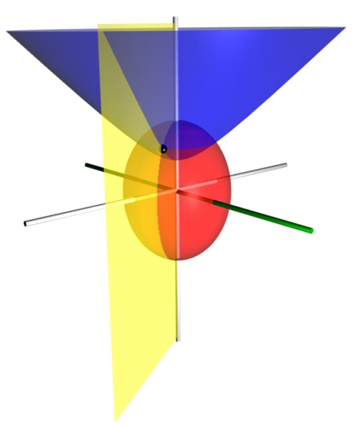
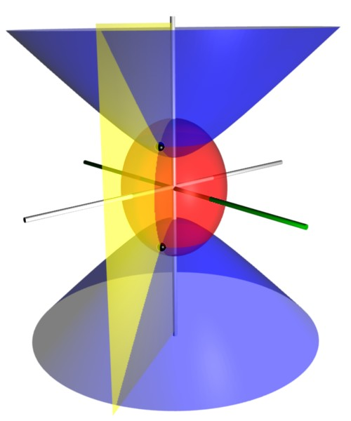
shows that surfaces of constant \mu form prolate spheroids, since they are ellipses rotated about the axis joining their foci. Similarly, the hyperbolic trigonometric identity

: \frac{z^2}{a^2 \cos^2 \nu} - \frac{x^2 + y^2}{a^2 \sin^2 \nu} = \cosh^2 \mu - \sinh^2 \mu = 1

shows that surfaces of constant \nu form hyperboloids of revolution.

The distances from the foci located at (x, y, z) = (0, 0, \pm a) are

: r_\pm = \sqrt{x^2 + y^2 + (z \mp a)^2} = a(\cosh \mu \mp \cos \nu).

Scale factors

The scale factors for the elliptic coordinates (\mu, \nu) are equal

: h_\mu = h_\nu = a\sqrt{\sinh^2\mu + \sin^2\nu}

whereas the azimuthal scale factor is

: h_\varphi = a \sinh\mu \sin\nu,

resulting in a metric of

: \begin{align} ds^2 &= h_\mu^2 d\mu^2 + h_\nu^2 d\nu^2 + h_\varphi^2 d\varphi^2 \ &= a^2 \left[ (\sinh^2\mu + \sin^2\nu) d\mu^2 + (\sinh^2\mu + \sin^2\nu) d\nu^2 + (\sinh^2\mu \sin^2\nu) d\varphi^2 \right]. \end{align}

Consequently, an infinitesimal volume element equals

: dV = a^3 \sinh\mu \sin\nu ( \sinh^2 \mu + \sin^2 \nu) , d\mu , d\nu , d\varphi

and the Laplacian can be written

: \begin{align} \nabla^2 \Phi = {} & \frac{1}{a^2 (\sinh^2 \mu + \sin^2 \nu)} \left[ \frac{\partial^2 \Phi}{\partial \mu^2} + \frac{\partial^2 \Phi}{\partial \nu^2} + \coth \mu \frac{\partial \Phi}{\partial \mu} + \cot \nu \frac{\partial \Phi}{\partial \nu} \right] \[6pt] & {} + \frac{1}{a^2 \sinh^2 \mu \sin^2\nu} \frac{\partial^2 \Phi}{\partial \varphi^2} \end{align}

Other differential operators such as \nabla \cdot \mathbf{F} and \nabla \times \mathbf{F} can be expressed in the coordinates (\mu, \nu, \varphi) by substituting the scale factors into the general formulae found in orthogonal coordinates.

Alternative definition(1)

An alternative and geometrically intuitive set of prolate spheroidal coordinates (\sigma, \tau, \phi) are sometimes used, where \sigma = \cosh \mu and \tau = \cos \nu. Hence, the curves of constant \sigma are prolate spheroids, whereas the curves of constant \tau are hyperboloids of revolution. The coordinate \tau belongs to the interval [−1, 1], whereas the \sigma coordinate must be greater than or equal to one.

The coordinates \sigma and \tau have a simple relation to the distances to the foci F_{1} and F_{2}. For any point in the plane, the sum d_{1}+d_{2} of its distances to the foci equals 2a\sigma, whereas their difference d_{1}-d_{2} equals 2a\tau. Thus, the distance to F_{1} is a(\sigma+\tau), whereas the distance to F_{2} is a(\sigma-\tau). (Recall that F_{1} and F_{2} are located at z=-a and z=+a, respectively.) This gives the following expressions for \sigma, \tau, and \varphi:

: \sigma = \frac 1 {2a} \left(\sqrt{x^2+y^2+(z+a)^2}+\sqrt{x^2+y^2+(z-a)^2}\right)

: \tau = \frac 1 {2a} \left(\sqrt{x^2+y^2+(z+a)^2}-\sqrt{x^2+y^2+(z-a)^2}\right)

: \varphi = \arctan\left(\frac y x \right)

Unlike the analogous oblate spheroidal coordinates, the prolate spheroid coordinates (σ, τ, φ) are not degenerate; in other words, there is a unique, reversible correspondence between them and the Cartesian coordinates

: x = a \sqrt{(\sigma^2 - 1) (1 - \tau^2)} \cos \varphi

: y = a \sqrt{(\sigma^2 - 1) (1 - \tau^2)} \sin \varphi

: z = a\ \sigma\ \tau

Alternative scale factors

The scale factors for the alternative elliptic coordinates (\sigma, \tau, \varphi) are

: h_{\sigma} = a\sqrt{\frac{\sigma^{2} - \tau^{2}}{\sigma^{2} - 1}}

: h_{\tau} = a\sqrt{\frac{\sigma^{2} - \tau^{2}}{1 - \tau^{2}}}

while the azimuthal scale factor is now

: h_\varphi = a \sqrt{\left( \sigma^{2} - 1 \right) \left( 1 - \tau^{2} \right)}

Hence, the infinitesimal volume element becomes

: dV = a^3 (\sigma^2 - \tau^2) , d\sigma , d\tau , d\varphi

and the Laplacian equals

: \begin{align} \nabla^2 \Phi = {} & \frac{1}{a^2 (\sigma^2 - \tau^2)} \left{ \frac{\partial}{\partial \sigma} \left[ \left( \sigma^2 - 1 \right) \frac{\partial \Phi}{\partial \sigma} \right] + \frac{\partial}{\partial \tau} \left[ (1 - \tau^2) \frac{\partial \Phi}{\partial \tau} \right] \right} \ & {} + \frac{1}{a^2 (\sigma^2 - 1) (1 - \tau^2)} \frac{\partial^2 \Phi}{\partial \varphi^2} \end{align}

Other differential operators such as \nabla \cdot \mathbf{F} and \nabla \times \mathbf{F} can be expressed in the coordinates (\sigma, \tau) by substituting the scale factors into the general formulae found in orthogonal coordinates.

As is the case with spherical coordinates, Laplace's equation may be solved by the method of separation of variables to yield solutions in the form of prolate spheroidal harmonics, which are convenient to use when boundary conditions are defined on a surface with a constant prolate spheroidal coordinate (See Smythe, 1968).

Alternative definition(2)

Prolate spheroidal coordinates (η, θ, ϕ; d){{cite journal | url-access=subscription

\begin{aligned} x &= \sqrt{\eta^2 - d^2},\sin\theta\cos\phi,\ y &= \sqrt{\eta^2 - d^2},\sin\theta\sin\phi,\ z &= \eta,\cos\theta, \end{aligned}

where

0\le\theta\le\pi,\quad 0\le\phi

and 𝑑0 denotes the focal distance (half the separation between the foci of a cross-sectional ellipse). Note that if d=0, the cross-section is a circle, and coordinates become those for a sphere. The normal to the surface at each point is η, which has its length equal to the semi-major axis of a cross-sectional ellipse.

References

Bibliography

No angles convention

• Uses ξ1 = a cosh μ, ξ2 = sin ν, and ξ3 = cos φ.
• Same as Morse & Feshbach (1953), substituting u**k for ξ**k.
• Uses coordinates ξ = cosh μ, η = sin ν, and φ.

Angle convention

• Korn and Korn use the (μ, ν, φ) coordinates, but also introduce the degenerate (σ, τ, φ) coordinates.
• Similar to Korn and Korn (1961), but uses colatitude θ = 90° - ν instead of latitude ν.
• Moon and Spencer use the colatitude convention θ = 90° − ν, and rename φ as ψ.

Unusual convention

• Treats the prolate spheroidal coordinates as a limiting case of the general ellipsoidal coordinates. Uses (ξ, η, ζ) coordinates that have the units of distance squared.

References

1. (21 May 2019). "A review on non-relativistic, fully numerical electronic structure calculations on atoms and diatomic molecules". Int. J. Quantum Chem..