Padua points

The four families

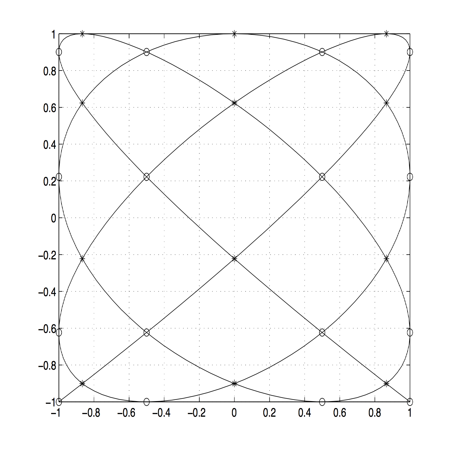
We can see the Padua point as a "sampling" of a parametric curve, called generating curve, which is slightly different for each of the four families, so that the points for interpolation degree n and family s can be defined as

:\text{Pad}_n^s=\lbrace\mathbf{\xi}=(\xi_1,\xi_2)\rbrace=\left\lbrace\gamma_s\left(\frac{k\pi}{n(n+1)}\right),k=0,\ldots,n(n+1)\right\rbrace.

Actually, the Padua points lie exactly on the self-intersections of the curve, and on the intersections of the curve with the boundaries of the square [-1,1]^2. The cardinality of the set \operatorname{Pad}_n^s is |\operatorname{Pad}_n^s| = \frac{(n+1)(n+2)}{2}. Moreover, for each family of Padua points, two points lie on consecutive vertices of the square [-1,1]^2, 2n-1 points lie on the edges of the square, and the remaining points lie on the self-intersections of the generating curve inside the square.

The four generating curves are closed parametric curves in the interval [0,2\pi], and are a special case of Lissajous curves.

The first family

The generating curve of Padua points of the first family is

:\gamma_1(t)=[-\cos((n+1)t),-\cos(nt)],\quad t\in [0,\pi].

If we sample it as written above, we have:

:\operatorname{Pad}_n^1=\lbrace\mathbf{\xi}=(\mu_j,\eta_k), 0\le j\le n; 1\le k\le\lfloor\frac{n}{2}\rfloor+1+\delta_j\rbrace, where \delta_j=0 when n is even or odd but j is even, \delta_j=1 if n and k are both odd

with

:\mu_j=\cos\left(\frac{j\pi}{n}\right), \eta_k= \begin{cases} \cos\left(\frac{(2k-2)\pi}{n+1}\right) & j\mbox{ odd} \ \cos\left(\frac{(2k-1)\pi}{n+1}\right) & j\mbox{ even.} \end{cases}

From this follows that the Padua points of first family will have two vertices on the bottom if n is even, or on the left if n is odd.

The second family

The generating curve of Padua points of the second family is

:\gamma_2(t)=[-\cos(nt),-\cos((n+1)t)],\quad t\in [0,\pi],

which leads to have vertices on the left if n is even and on the bottom if n is odd.

The third family

The generating curve of Padua points of the third family is

:\gamma_3(t)=[\cos((n+1)t),\cos(nt)],\quad t\in [0,\pi],

which leads to have vertices on the top if n is even and on the right if n is odd.

The fourth family

The generating curve of Padua points of the fourth family is

:\gamma_4(t)=[\cos(nt),\cos((n+1)t)],\quad t\in [0,\pi],

which leads to have vertices on the right if n is even and on the top if n is odd.

The interpolation formula

The explicit representation of their fundamental Lagrange polynomial is based on the reproducing kernel K_n(\mathbf{x},\mathbf{y}), \mathbf{x}=(x_1,x_2) and \mathbf{y}=(y_1,y_2), of the space \Pi_n^2([-1,1]^2) equipped with the inner product

:\langle f,g\rangle =\frac{1}{\pi^2} \int_{[-1,1]^2} f(x_1,x_2)g(x_1,x_2)\frac{dx_1}{\sqrt{1-x_1^2}}\frac{dx_2}{\sqrt{1-x_2^2}}

defined by

:K_n(\mathbf{x},\mathbf{y})=\sum_{k=0}^n\sum_{j=0}^k \hat T_j(x_1)\hat T_{k-j}(x_2)\hat T_j(y_1)\hat T_{k-j}(y_2)

with \hat T_j representing the normalized Chebyshev polynomial of degree j (that is, \hat T_0=T_0 and \hat T_p=\sqrt{2}T_p, where T_p(\cdot)=\cos(p\arccos(\cdot)) is the classical Chebyshev polynomial of first kind of degree p). For the four families of Padua points, which we may denote by \operatorname{Pad}_n^s=\lbrace\mathbf{\xi}=(\xi_1,\xi_2)\rbrace, s=\lbrace 1,2,3,4\rbrace, the interpolation formula of order n of the function f\colon [-1,1]^2\to\mathbb{R}^2 on the generic target point \mathbf{x}\in [-1,1]^2 is then

: \mathcal{L}n^s f(\mathbf{x})=\sum{\mathbf{\xi}\in\operatorname{Pad}n^s}f(\mathbf{\xi})L^s{\mathbf\xi}(\mathbf{x})

where L^s_{\mathbf\xi}(\mathbf{x}) is the fundamental Lagrange polynomial

:L^s_{\mathbf\xi}(\mathbf{x})=w_{\mathbf\xi}(K_n(\mathbf\xi,\mathbf{x})-T_n(\xi_i)T_n(x_i)),\quad s=1,2,3,4,\quad i=2-(s\mod 2).

The weights w_{\mathbf\xi} are defined as

: w_{\mathbf\xi}=\frac{1}{n(n+1)}\cdot \begin{cases} \frac{1}{2}\text{ if }\mathbf\xi\text{ is a vertex point}\ 1\text{ if }\mathbf\xi\text{ is an edge point}\ 2\text{ if }\mathbf\xi\text{ is an interior point.} \end{cases}

References