From Surf Wiki (app.surf) — the open knowledge base
Lemniscate elliptic functions
Mathematical functions

Mathematical functions
In mathematics, the lemniscate elliptic functions are elliptic functions related to the arc length of the lemniscate of Bernoulli. They were first studied by Giulio Fagnano in 1718 and later by Leonhard Euler and Carl Friedrich Gauss, among others.
The lemniscate sine and lemniscate cosine functions, usually written with the symbols sl and cl (sometimes the symbols sinlem and coslem or sin lemn and cos lemn are used instead), are analogous to the trigonometric functions sine and cosine. While the trigonometric sine relates the arc length to the chord length in a unit-diameter circle NOTE: THE RHS IN THE FOLLOWING IS x, NOT 1 --x^2+y^2 = x, the lemniscate sine relates the arc length to the chord length of a lemniscate \bigl(x^2+y^2\bigr){}^2=x^2-y^2.
The lemniscate functions have periods related to a number called the lemniscate constant, the ratio of a lemniscate's perimeter to its diameter. This number is a quartic analog of the (quadratic) , ratio of perimeter to diameter of a circle.
As complex functions, sl and cl have a square period lattice (a multiple of the Gaussian integers) with fundamental periods {(1 + i)\varpi, (1 - i)\varpi}, and are a special case of two Jacobi elliptic functions on that lattice, \operatorname{sl} z = \operatorname{sn}(z; -1), \operatorname{cl} z = \operatorname{cd}(z; -1).
Similarly, the hyperbolic lemniscate sine slh and hyperbolic lemniscate cosine clh have a square period lattice with fundamental periods \bigl{\sqrt2\varpi, \sqrt2\varpi i\bigr}.
The lemniscate functions and the hyperbolic lemniscate functions are related to the Weierstrass elliptic function \wp (z;a,0).
Lemniscate sine and cosine functions
Definitions
The lemniscate functions sl and cl can be defined as the solution to the initial value problem:
:\frac{\mathrm{d}}{\mathrm{d}z} \operatorname{sl} z = \bigl(1 + \operatorname{sl}^2 z\bigr)\operatorname{cl}z,\ \frac{\mathrm{d}}{\mathrm{d}z} \operatorname{cl} z = -\bigl(1 + \operatorname{cl}^2 z\bigr)\operatorname{sl}z,\ \operatorname{sl} 0 = 0,\ \operatorname{cl} 0 = 1,
or equivalently as the inverses of an elliptic integral, the Schwarz–Christoffel map from the complex unit disk to a square with corners \big{\tfrac12\varpi, \tfrac12\varpi i, -\tfrac12\varpi, -\tfrac12\varpi i\big}\colon : z = \int_0^{\operatorname{sl} z}\frac{\mathrm{d}t}{\sqrt{1-t^4}} = \int_{\operatorname{cl} z}^1\frac{\mathrm{d}t}{\sqrt{1-t^4}}.
Beyond that square, the functions can be extended to the complex plane via analytic continuation by successive reflections.
By comparison, the circular sine and cosine can be defined as the solution to the initial value problem:
:\frac{\mathrm{d}}{\mathrm{d}z} \sin z = \cos z,\ \frac{\mathrm{d}}{\mathrm{d}z} \cos z = -\sin z,\ \sin 0 = 0,\ \cos 0 = 1,
or as inverses of a map from the upper half-plane to a half-infinite strip with real part between -\tfrac12\pi, \tfrac12\pi and positive imaginary part: : z = \int_0^{\sin z}\frac{\mathrm{d}t}{\sqrt{1-t^2}} = \int_{\cos z}^1\frac{\mathrm{d}t}{\sqrt{1-t^2}}.
Relation to the lemniscate constant
Main article: Lemniscate constant

The lemniscate functions have minimal real period , minimal imaginary period and fundamental complex periods (1+i)\varpi and (1-i)\varpi for a constant called the lemniscate constant,
:\varpi = 2\int_0^1\frac{\mathrm{d}t}{\sqrt{1-t^4}} = 2.62205\ldots
The lemniscate functions satisfy the basic relation \operatorname{cl}z = {\operatorname{sl}}\bigl(\tfrac12\varpi - z\bigr), analogous to the relation \cos z = {\sin}\bigl(\tfrac12\pi - z\bigr).
The lemniscate constant is a close analog of the circle constant , and many identities involving have analogues involving , as identities involving the trigonometric functions have analogues involving the lemniscate functions. For example, Viète's formula for can be written:
\frac2\pi = \sqrt\frac12 \cdot \sqrt{\frac12 + \frac12\sqrt\frac12} \cdot \sqrt{\frac12 + \frac12\sqrt{\frac12 + \frac12\sqrt\frac12}} \cdots
An analogous formula for is:
\frac2\varpi = \sqrt\frac12 \cdot \sqrt{\frac12 + \frac12 \bigg/ !\sqrt\frac12} \cdot \sqrt{\frac12 + \frac12 \Bigg/ !\sqrt{\frac12 + \frac12 \bigg/ !\sqrt\frac12}} \cdots
The Machin formula for is \tfrac14\pi = 4 \arctan \tfrac15 - \arctan \tfrac1{239}, and several similar formulas for can be developed using trigonometric angle sum identities, e.g. Euler's formula \tfrac14\pi = \arctan\tfrac12 + \arctan\tfrac13. Analogous formulas can be developed for , including the following found by Gauss: \tfrac12\varpi = 2 \operatorname{arcsl} \tfrac12 + \operatorname{arcsl} \tfrac7{23}.
The lemniscate and circle constants were found by Gauss to be related to each-other by the arithmetic-geometric mean :
\frac\pi\varpi = M{\left(1, \sqrt2!~\right)}
Argument identities
Zeros, poles and symmetries

The lemniscate functions cl and sl are even and odd functions, respectively, :\begin{aligned} \operatorname{cl}(-z) &= \operatorname{cl} z \[6mu] \operatorname{sl}(-z) &= - \operatorname{sl} z \end{aligned}
At translations of \tfrac12\varpi, cl and sl are exchanged, and at translations of \tfrac12i\varpi they are additionally rotated and reciprocated:
:\begin{aligned} {\operatorname{cl}}\bigl(z \pm \tfrac12\varpi\bigr) &= \mp\operatorname{sl} z,& {\operatorname{cl}}\bigl(z \pm \tfrac12i\varpi\bigr) &= \frac{\mp i}{\operatorname{sl} z} \[6mu] {\operatorname{sl}}\bigl(z \pm \tfrac12\varpi\bigr) &= \pm\operatorname{cl} z,& {\operatorname{sl}}\bigl(z \pm \tfrac12i\varpi\bigr) &= \frac{\pm i}{\operatorname{cl} z} \end{aligned}
Doubling these to translations by a unit-Gaussian-integer multiple of \varpi (that is, \pm \varpi or \pm i\varpi), negates each function, an involution:
:\begin{aligned} \operatorname{cl} (z + \varpi) &= \operatorname{cl} (z + i\varpi) = -\operatorname{cl} z \[4mu] \operatorname{sl} (z + \varpi) &= \operatorname{sl} (z + i\varpi) = -\operatorname{sl} z \end{aligned}
As a result, both functions are invariant under translation by an even-Gaussian-integer multiple of \varpi. That is, a displacement (a + bi)\varpi, with a + b = 2k for integers , , and .
:\begin{aligned} {\operatorname{cl}}\bigl(z + (1 + i)\varpi\bigr) &= {\operatorname{cl}} \bigl(z + (1 - i)\varpi\bigr) = \operatorname{cl} z \[4mu] {\operatorname{sl}}\bigl(z + (1 + i)\varpi\bigr) &= {\operatorname{sl}} \bigl(z + (1 - i)\varpi\bigr) = \operatorname{sl} z \end{aligned}
This makes them elliptic functions (doubly periodic meromorphic functions in the complex plane) with a diagonal square period lattice of fundamental periods (1 + i)\varpi and (1 - i)\varpi. Elliptic functions with a square period lattice are more symmetrical than arbitrary elliptic functions, following the symmetries of the square.
Reflections and quarter-turn rotations of lemniscate function arguments have simple expressions:
:\begin{aligned} \operatorname{cl} \bar{z} &= \overline{\operatorname{cl} z} \[6mu] \operatorname{sl} \bar{z} &= \overline{\operatorname{sl} z} \[4mu] \operatorname{cl} iz &= \frac{1}{\operatorname{cl} z} \[6mu] \operatorname{sl} iz &= i \operatorname{sl} z \end{aligned}
The sl function has simple zeros at Gaussian integer multiples of , complex numbers of the form a\varpi + b\varpi i for integers and . It has simple poles at Gaussian half-integer multiples of , complex numbers of the form \bigl(a + \tfrac12\bigr)\varpi + \bigl(b + \tfrac12\bigr)\varpi i, with residues (-1)^{a-b+1}i. The cl function is reflected and offset from the sl function, \operatorname{cl}z = {\operatorname{sl}}\bigl(\tfrac12\varpi - z\bigr). It has zeros for arguments \bigl(a + \tfrac12\bigr)\varpi + b\varpi i and poles for arguments a\varpi + \bigl(b + \tfrac12\bigr)\varpi i, with residues (-1)^{a-b}i.
Also :\operatorname{sl}z=\operatorname{sl}w\leftrightarrow z=(-1)^{m+n}w+(m+ni)\varpi for some m,n\in\mathbb{Z} and :\operatorname{sl}((1\pm i)z)=(1\pm i)\frac{\operatorname{sl}z}{\operatorname{sl}'z}. The last formula is a special case of complex multiplication. Analogous formulas can be given for \operatorname{sl}((n+mi)z) where n+mi is any Gaussian integer – the function \operatorname{sl} has complex multiplication by \mathbb{Z}[i].
There are also infinite series reflecting the distribution of the zeros and poles of sl: :\frac{1}{\operatorname{sl}z}=\sum_{(n,k)\in\mathbb{Z}^2}\frac{(-1)^{n+k}}{z+n\varpi+k\varpi i} :\operatorname{sl}z=-i\sum_{(n,k)\in\mathbb{Z}^2}\frac{(-1)^{n+k}}{z+(n+1/2)\varpi +(k+1/2)\varpi i}.
Pythagorean-like identity
_=_a(1_-_x²y²)_for_various_values_of_a.png)
The lemniscate functions satisfy a Pythagorean-like identity: :\operatorname{cl^2} z + \operatorname{sl^2} z + \operatorname{cl^2} z , \operatorname{sl^2} z = 1
As a result, the parametric equation (x, y) = (\operatorname{cl} t, \operatorname{sl} t) parametrizes the quartic curve x^2 + y^2 + x^2y^2 = 1.
This identity can alternately be rewritten:
:\bigl(1 + \operatorname{cl^2} z\bigr) \bigl(1+\operatorname{sl^2} z\bigr) = 2
:\operatorname{cl^2} z = \frac{1 - \operatorname{sl^2} z}{1 + \operatorname{sl^2} z},\quad \operatorname{sl^2} z = \frac{1 - \operatorname{cl^2} z}{1 + \operatorname{cl^2} z}
Defining a tangent-sum operator as a \oplus b \mathrel{:=} \tan(\arctan a + \arctan b) = \frac{a+b}{1-ab}, gives:
:\operatorname{cl^2} z \oplus \operatorname{sl^2} z = 1.
Derivatives and integrals
The derivatives are as follows:
:\begin{aligned} \frac{\mathrm{d}}{\mathrm{d}z}\operatorname{cl} z = \operatorname{cl'}z &= -\bigl(1 + \operatorname{cl^2} z\bigr)\operatorname{sl}z=-\frac{2\operatorname{sl}z}{\operatorname{sl}^2z+1} \ \operatorname{cl'^2} z &= 1 - \operatorname{cl^4} z \[5mu]
\frac{\mathrm{d}}{\mathrm{d}z}\operatorname{sl} z = \operatorname{sl'}z &= \bigl(1 + \operatorname{sl^2} z\bigr)\operatorname{cl}z=\frac{2\operatorname{cl}z}{\operatorname{cl}^2z+1}\ \operatorname{sl'^2} z &= 1 - \operatorname{sl^4} z\end{aligned}
:\begin{align}\frac{\mathrm d}{\mathrm dz},\tilde{\operatorname{cl}},z&=-2,\tilde{\operatorname{sl}},z,\operatorname{cl}z-\frac{\tilde{\operatorname{sl}},z}{\operatorname{cl}z}\
\frac{\mathrm d}{\mathrm dz},\tilde{\operatorname{sl}},z&=2,\tilde{\operatorname{cl}},z,\operatorname{cl}z-\frac{\tilde{\operatorname{cl}},z}{\operatorname{cl}z}
\end{align}
The second derivatives of lemniscate sine and lemniscate cosine are their negative duplicated cubes:
:\frac{\mathrm{d}^2}{\mathrm{d}z^2}\operatorname{cl}z = -2\operatorname{cl^3}z
:\frac{\mathrm{d}^2}{\mathrm{d}z^2}\operatorname{sl}z = -2\operatorname{sl^3}z
The lemniscate functions can be integrated using the inverse tangent function:
:\begin{align}\int\operatorname{cl} z \mathop{\mathrm{d}z}& = \arctan \operatorname{sl} z + C\ \int\operatorname{sl} z \mathop{\mathrm{d}z}& = -\arctan \operatorname{cl} z + C\ \int\tilde{\operatorname{cl}},z,\mathrm dz&=\frac{\tilde{\operatorname{sl}},z}{\operatorname{cl}z}+C\ \int\tilde{\operatorname{sl}},z,\mathrm dz&=-\frac{\tilde{\operatorname{cl}},z}{\operatorname{cl}z}+C\end{align}
Argument sum and multiple identities
Like the trigonometric functions, the lemniscate functions satisfy argument sum and difference identities. The original identity used by Fagnano for bisection of the lemniscate was:
: \operatorname{sl}(u+v) = \frac{\operatorname{sl}u,\operatorname{sl'}v + \operatorname{sl}v,\operatorname{sl'}u} {1 + \operatorname{sl^2}u, \operatorname{sl^2}v}
The derivative and Pythagorean-like identities can be used to rework the identity used by Fagano in terms of sl and cl. Defining a tangent-sum operator a \oplus b \mathrel{:=} \tan(\arctan a + \arctan b) and tangent-difference operator a \ominus b \mathrel{:=} a \oplus (-b), the argument sum and difference identities can be expressed as:
:\begin{aligned} \operatorname{cl}(u+v) &= \operatorname{cl}u,\operatorname{cl}v \ominus \operatorname{sl}u, \operatorname{sl}v = \frac{\operatorname{cl}u, \operatorname{cl}v - \operatorname{sl}u, \operatorname{sl}v} {1 + \operatorname{sl}u, \operatorname{cl}u, \operatorname{sl}v, \operatorname{cl}v} \[2mu] \operatorname{cl}(u-v) &= \operatorname{cl}u,\operatorname{cl}v \oplus \operatorname{sl}u, \operatorname{sl}v \[2mu] \operatorname{sl}(u+v) &= \operatorname{sl}u,\operatorname{cl}v \oplus \operatorname{cl}u,\operatorname{sl}v = \frac{\operatorname{sl}u, \operatorname{cl}v + \operatorname{cl}u, \operatorname{sl}v} {1 - \operatorname{sl}u, \operatorname{cl}u, \operatorname{sl}v, \operatorname{cl}v} \[2mu] \operatorname{sl}(u-v) &= \operatorname{sl}u,\operatorname{cl}v \ominus \operatorname{cl}u,\operatorname{sl}v \end{aligned}
These resemble their trigonometric analogs:
:\begin{aligned} \cos(u \pm v) &= \cos u,\cos v \mp \sin u,\sin v \[6mu] \sin(u \pm v) &= \sin u,\cos v \pm \cos u,\sin v \end{aligned}
In particular, to compute the complex-valued functions in real components,
:\begin{aligned} \operatorname{cl}(x + iy) &= \frac{\operatorname{cl}x - i \operatorname{sl}x, \operatorname{sl}y, \operatorname{cl}y} {\operatorname{cl}y + i \operatorname{sl}x, \operatorname{cl}x, \operatorname{sl}y} \[4mu] &= \frac{\operatorname{cl}x,\operatorname{cl}y\left(1 - \operatorname{sl}^2x,\operatorname{sl}^2y\right)}{\operatorname{cl}^2y + \operatorname{sl}^2x,\operatorname{cl}^2x,\operatorname{sl}^2y}
- i \frac{\operatorname{sl}x,\operatorname{sl}y\left(\operatorname{cl}^2x + \operatorname{cl}^2y\right)}{\operatorname{cl}^2y + \operatorname{sl}^2x,\operatorname{cl}^2x,\operatorname{sl}^2y} \[12mu] \operatorname{sl}(x + iy) &= \frac{\operatorname{sl}x + i \operatorname{cl}x, \operatorname{sl}y, \operatorname{cl}y} {\operatorname{cl}y - i \operatorname{sl}x, \operatorname{cl}x, \operatorname{sl}y } \[4mu] &= \frac{\operatorname{sl}x,\operatorname{cl}y\left(1 - \operatorname{cl}^2x,\operatorname{sl}^2y\right)}{\operatorname{cl}^2y + \operatorname{sl}^2x,\operatorname{cl}^2x,\operatorname{sl}^2y}
- i \frac{\operatorname{cl}x,\operatorname{sl}y\left(\operatorname{sl}^2x + \operatorname{cl}^2y\right)}{\operatorname{cl}^2y + \operatorname{sl}^2x,\operatorname{cl}^2x,\operatorname{sl}^2y} \end{aligned}
Gauss discovered that :\frac{\operatorname{sl}(u-v)}{\operatorname{sl}(u+v)}=\frac{\operatorname{sl}((1+i)u)-\operatorname{sl}((1+i)v)}{\operatorname{sl}((1+i)u)+\operatorname{sl}((1+i)v)} where u,v\in\mathbb{C} such that both sides are well-defined.
Also :\operatorname{sl}(u+v)\operatorname{sl}(u-v)=\frac{\operatorname{sl}^2u-\operatorname{sl}^2v}{1+\operatorname{sl}^2u\operatorname{sl}^2v} where u,v\in\mathbb{C} such that both sides are well-defined; this resembles the trigonometric analog :\sin (u+v)\sin (u-v)=\sin^2u-\sin^2v.
Bisection formulas:
: \operatorname{cl}^2 \tfrac12x = \frac{1+\operatorname{cl}x \sqrt{1+\operatorname{sl}^2x}}{1 + \sqrt{1+\operatorname{sl}^2x}}
: \operatorname{sl}^2 \tfrac12x = \frac{1-\operatorname{cl}x\sqrt{1+\operatorname{sl}^2x}}{1 + \sqrt{1+\operatorname{sl}^2x}}
Duplication formulas:
: \operatorname{cl} 2x = \frac{-1+2,\operatorname{cl}^2x + \operatorname{cl}^4x}{1+2,\operatorname{cl}^2x - \operatorname{cl}^4x}
: \operatorname{sl} 2x = 2,\operatorname{sl}x,\operatorname{cl}x\frac{1+\operatorname{sl}^2x}{1+\operatorname{sl}^4x}
Triplication formulas:
: \operatorname{cl} 3x = \frac{-3,\operatorname{cl}x + 6,\operatorname{cl}^5x + \operatorname{cl}^9x}{1+6,\operatorname{cl}^4x - 3,\operatorname{cl}^8x}
: \operatorname{sl} 3x = \frac{\color{red}{3},\color{black}{\operatorname{sl}x -, }\color{green}{6},\color{black}{\operatorname{sl}^5x -,}\color{blue}{1},\color{black}{ \operatorname{sl}^9x}}{\color{blue}{1},\color{black}{+,},\color{green}{6},\color{black}{\operatorname{sl}^4x -, }\color{red}{3},\color{black}{\operatorname{sl}^8x}}
Note the "reverse symmetry" of the coefficients of numerator and denominator of \operatorname{sl}3x. This phenomenon can be observed in multiplication formulas for \operatorname{sl}\beta x where \beta=m+ni whenever m,n\in\mathbb{Z} and m+n is odd.
Lemnatomic polynomials
Let L be the lattice :L=\mathbb{Z}(1+i)\varpi +\mathbb{Z}(1-i)\varpi. Furthermore, let K=\mathbb{Q}(i), \mathcal{O}=\mathbb{Z}[i], z\in\mathbb{C}, \beta=m+in, \gamma=m'+in' (where m,n,m',n'\in\mathbb{Z}), m+n be odd, m'+n' be odd, \gamma\equiv 1,\operatorname{mod}, 2(1+i) and \operatorname{sl} \beta z=M_\beta (\operatorname{sl}z). Then :M_\beta (x)=i^\varepsilon x \frac{P_\beta (x^4)}{Q_\beta (x^4)} for some coprime polynomials P_\beta (x), Q_\beta (x)\in \mathcal{O}[x] and some \varepsilon\in {0,1,2,3} where :xP_\beta (x^4)=\prod_{\gamma |\beta}\Lambda_\gamma (x) and :\Lambda_\beta (x)=\prod_{[\alpha]\in (\mathcal{O}/\beta\mathcal{O})^\times}(x-\operatorname{sl}\alpha\delta_\beta) where \delta_\beta is any \beta-torsion generator (i.e. \delta_\beta \in (1/\beta)L and [\delta_\beta]\in (1/\beta)L/L generates (1/\beta)L/L as an \mathcal{O}-module). Examples of \beta-torsion generators include 2\varpi/\beta and (1+i)\varpi/\beta. The polynomial \Lambda_\beta (x)\in\mathcal{O}[x] is called the \beta-th lemnatomic polynomial. It is monic and is irreducible over K. The lemnatomic polynomials are the "lemniscate analogs" of the cyclotomic polynomials, :\Phi_k(x)=\prod_{[a]\in (\mathbb{Z}/k\mathbb{Z})^\times}(x-\zeta_k^a).
The \beta-th lemnatomic polynomial \Lambda_\beta(x) is the minimal polynomial of \operatorname{sl}\delta_\beta in K[x]. For convenience, let \omega_{\beta}=\operatorname{sl}(2\varpi/\beta) and \tilde{\omega}{\beta}=\operatorname{sl}((1+i)\varpi/\beta). So for example, the minimal polynomial of \omega_5 (and also of \tilde{\omega}5) in K[x] is :\Lambda_5(x)=x^{16}+52x^{12}-26x^8-12x^4+1, and :\omega_5=\sqrt[4]{-13+6\sqrt{5}+2\sqrt{85-38\sqrt{5}}} :\tilde{\omega}5=\sqrt[4]{-13-6\sqrt{5}+2\sqrt{85+38\sqrt{5}}} (an equivalent expression is given in the table below). Another example is :\Lambda{-1+2i}(x)=x^4-1+2i which is the minimal polynomial of \omega{-1+2i} (and also of \tilde{\omega}{-1+2i}) in K[x].
If p is prime and \beta is positive and odd, then :\operatorname{deg}\Lambda_{\beta}=\beta^2\prod_{p|\beta}\left(1-\frac{1}{p}\right)\left(1-\frac{(-1)^{(p-1)/2}}{p}\right) which can be compared to the cyclotomic analog :\operatorname{deg}\Phi_{k}=k\prod_{p|k}\left(1-\frac{1}{p}\right).
Specific values
Just as for the trigonometric functions, values of the lemniscate functions can be computed for divisions of the lemniscate into parts of equal length, using only basic arithmetic and square roots, if and only if is of the form n = 2^kp_1p_2\cdots p_m where is a non-negative integer and each (if any) is a distinct Fermat prime.
| n | \operatorname{cl}n\varpi | \operatorname{sl}n\varpi |
|---|---|---|
| 1 | -1 | 0 |
| \tfrac{5}{6} | -\sqrt[4]{2\sqrt{3}-3} | \tfrac12\bigl(\sqrt{3}+1-\sqrt[4]{12}\bigr) |
| \tfrac{3}{4} | -\sqrt{\sqrt2-1} | \sqrt{\sqrt2-1} |
| \tfrac{2}{3} | -\tfrac12\bigl(\sqrt{3}+1-\sqrt[4]{12}\bigr) | \sqrt[4]{2\sqrt{3}-3} |
| \tfrac{1}{2} | 0 | 1 |
| \tfrac{1}{3} | \tfrac12\bigl(\sqrt{3}+1-\sqrt[4]{12}\bigr) | \sqrt[4]{2\sqrt{3}-3} |
| \tfrac{1}{4} | \sqrt{\sqrt2-1} | \sqrt{\sqrt2-1} |
| \tfrac{1}{6} | \sqrt[4]{2\sqrt{3}-3} | \tfrac12\bigl(\sqrt{3}+1-\sqrt[4]{12}\bigr) |
Relation to geometric shapes
Arc length of Bernoulli's lemniscate

\mathcal{L}, the lemniscate of Bernoulli with unit distance from its center to its furthest point (i.e. with unit "half-width"), is essential in the theory of the lemniscate elliptic functions. It can be characterized in at least three ways:
Angular characterization: Given two points A and B which are unit distance apart, let B' be the reflection of B about A. Then \mathcal{L} is the closure of the locus of the points P such that |APB-APB'| is a right angle.
Focal characterization: \mathcal{L} is the locus of points in the plane such that the product of their distances from the two focal points F_1 = \bigl({-\tfrac1\sqrt2},0\bigr) and F_2 = \bigl(\tfrac1\sqrt2,0\bigr) is the constant \tfrac12.
Explicit coordinate characterization: \mathcal{L} is a quartic curve satisfying the polar equation r^2 = \cos 2\theta or the Cartesian equation \bigl(x^2+y^2\bigr){}^2=x^2-y^2.
The perimeter of \mathcal{L} is 2\varpi.
The points on \mathcal{L} at distance r from the origin are the intersections of the circle x^2+y^2=r^2 and the hyperbola x^2-y^2=r^4. The intersection in the positive quadrant has Cartesian coordinates: :\big(x(r), y(r)\big) = \biggl(!\sqrt{\tfrac12r^2\bigl(1 + r^2\bigr)},, \sqrt{\tfrac12r^2\bigl(1 - r^2\bigr)},\biggr).
Using this parametrization with r \in [0, 1] for a quarter of \mathcal{L}, the arc length from the origin to a point \big(x(r), y(r)\big) is: :\begin{aligned} &\int_0^r \sqrt{x'(t)^2 + y'(t)^2} \mathop{\mathrm{d}t} \ & \quad {}= \int_0^r \sqrt{\frac{(1+2t^2)^2}{2(1+t^2)} + \frac{(1-2t^2)^2}{2(1-t^2)}} \mathop{\mathrm{d}t} \[6mu] & \quad {}= \int_0^r \frac{\mathrm{d}t}{\sqrt{1-t^4}} \[6mu] & \quad {}= \operatorname{arcsl} r. \end{aligned}
Likewise, the arc length from (1,0) to \big(x(r), y(r)\big) is: :\begin{aligned} &\int_r^1 \sqrt{x'(t)^2 + y'(t)^2} \mathop{\mathrm{d}t} \ & \quad {}= \int_r^1 \frac{\mathrm{d}t}{\sqrt{1-t^4}} \[6mu] & \quad {}= \operatorname{arccl} r = \tfrac12\varpi - \operatorname{arcsl} r. \end{aligned}
Or in the inverse direction, the lemniscate sine and cosine functions give the distance from the origin as functions of arc length from the origin and the point (1,0), respectively.
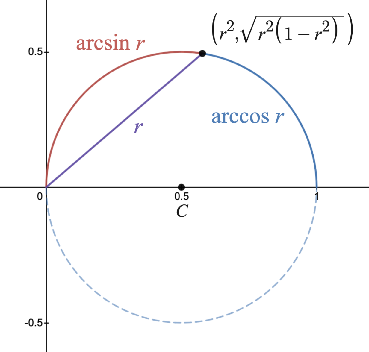
Analogously, the circular sine and cosine functions relate the chord length to the arc length for the unit diameter circle with polar equation r = \cos \theta or Cartesian equation x^2 + y^2 = x, using the same argument above but with the parametrization: :\big(x(r), y(r)\big) = \biggl(r^2,, \sqrt{r^2\bigl(1-r^2\bigr)},\biggr).
Alternatively, just as the unit circle x^2+y^2=1 is parametrized in terms of the arc length s from the point (1,0) by
:(x(s),y(s))=(\cos s,\sin s),
\mathcal{L} is parametrized in terms of the arc length s from the point (1,0) by
:(x(s),y(s))=\left(\frac{\operatorname{cl}s}{\sqrt{1+\operatorname{sl}^2 s}},\frac{\operatorname{sl}s\operatorname{cl}s}{\sqrt{1+\operatorname{sl}^2 s}}\right)=\left(\tilde{\operatorname{cl}},s,\tilde{\operatorname{sl}},s\right).
The notation \tilde{\operatorname{cl}},,\tilde{\operatorname{sl}} is used solely for the purposes of this article; in references, notation for general Jacobi elliptic functions is used instead.
The lemniscate integral and lemniscate functions satisfy an argument duplication identity discovered by Fagnano in 1718:
:\int_0^z \frac{\mathrm{d}t}{\sqrt{1 - t^4}} = 2 \int_0^u \frac{\mathrm{d}t}{\sqrt{1 - t^4}}, \quad \text{if } z = \frac{2u\sqrt{1 - u^4}}{1 + u^4} \text{ and } 0\le u\le\sqrt{\sqrt{2}-1}.
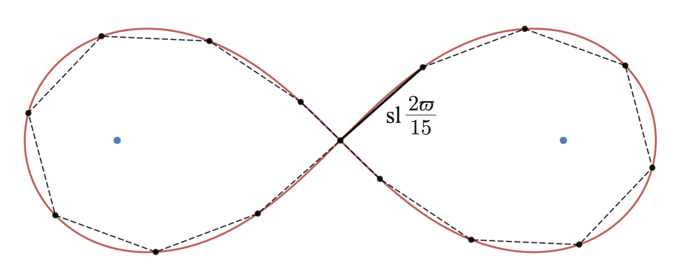
Later mathematicians generalized this result. Analogously to the constructible polygons in the circle, the lemniscate can be divided into sections of equal arc length using only straightedge and compass if and only if is of the form n = 2^kp_1p_2\cdots p_m where is a non-negative integer and each (if any) is a distinct Fermat prime. The "if" part of the theorem was proved by Niels Abel in 1827–1828, and the "only if" part was proved by Michael Rosen in 1981. Equivalently, the lemniscate can be divided into sections of equal arc length using only straightedge and compass if and only if \varphi (n) is a power of two (where \varphi is Euler's totient function). The lemniscate is not assumed to be already drawn, as that would go against the rules of straightedge and compass constructions; instead, it is assumed that we are given only two points by which the lemniscate is defined, such as its center and radial point (one of the two points on the lemniscate such that their distance from the center is maximal) or its two foci.
Let r_j=\operatorname{sl}\dfrac{2j\varpi}{n}. Then the -division points for \mathcal{L} are the points
:\left(r_j\sqrt{\tfrac12\bigl(1+r_j^2\bigr)},\ (-1)^{\left\lfloor 4j/n\right\rfloor} \sqrt{\tfrac12r_j^2\bigl(1-r_j^2\bigr)}\right),\quad j\in{1,2,\ldots ,n}
where \lfloor\cdot\rfloor is the floor function. See below for some specific values of \operatorname{sl}\dfrac{2\varpi}{n}.
Arc length of rectangular elastica

The inverse lemniscate sine also describes the arc length relative to the coordinate of the rectangular elastica. This curve has coordinate and arc length: :y = \int_x^1 \frac{t^2\mathop{\mathrm{d}t}}{\sqrt{1 - t^4}},\quad s = \operatorname{arcsl} x = \int_0^x \frac{\mathrm{d}t}{\sqrt{1 - t^4}}
The rectangular elastica solves a problem posed by Jacob Bernoulli, in 1691, to describe the shape of an idealized flexible rod fixed in a vertical orientation at the bottom end, and pulled down by a weight from the far end until it has been bent horizontal. Bernoulli's proposed solution established Euler–Bernoulli beam theory, further developed by Euler in the 18th century.
Elliptic characterization

Let C be a point on the ellipse x^2+2y^2=1 in the first quadrant and let D be the projection of C on the unit circle x^2+y^2=1. The distance r between the origin A and the point C is a function of \varphi (the angle BAC where B=(1,0); equivalently the length of the circular arc BD). The parameter u is given by :u=\int_0^{\varphi}r(\theta), \mathrm d\theta=\int_0^{\varphi}\frac{\mathrm d\theta}{\sqrt{1+\sin^2\theta}}. If E is the projection of D on the x-axis and if F is the projection of C on the x-axis, then the lemniscate elliptic functions are given by :\operatorname{cl}u=\overline{AF}, \quad \operatorname{sl}u=\overline{DE}, :\tilde{\operatorname{cl}}, u=\overline{AF}\overline{AC}, \quad \tilde{\operatorname{sl}}, u=\overline{AF}\overline{FC}.
Series Identities
Power series
The power series expansion of the lemniscate sine at the origin is :\operatorname{sl}z=\sum_{n=0}^\infty a_n z^n=z-12\frac{z^5}{5!}+3024\frac{z^9}{9!}-4390848\frac{z^{13}}{13!}+\cdots,\quad |z| where the coefficients a_n are determined as follows: :n\not\equiv 1\pmod 4\implies a_n=0, :a_1=1,, \forall n\in\mathbb{N}0:,a{n+2}=-\frac{2}{(n+1)(n+2)}\sum_{i+j+k=n}a_ia_ja_k
where i+j+k=n stands for all three-term compositions of n. For example, to evaluate a_{13}, it can be seen that there are only six compositions of 13-2=11 that give a nonzero contribution to the sum: 11=9+1+1=1+9+1=1+1+9 and 11=5+5+1=5+1+5=1+5+5, so :a_{13}=-\tfrac{2}{12\cdot 13}(a_9a_1a_1+a_1a_9a_1+a_1a_1a_9+a_5a_5a_1+a_5a_1a_5+a_1a_5a_5)=-\tfrac{11}{15600}.
The expansion can be equivalently written as :\operatorname{sl}z=\sum_{n=0}^\infty p_{2n} \frac{z^{4n+1}}{(4n+1)!},\quad \left|z\right| where :p_{n+2}=-12\sum_{j=0}^n\binom{2n+2}{2j+2}p_{n-j}\sum_{k=0}^j \binom{2j+1}{2k+1}p_k p_{j-k},\quad p_0=1,, p_1=0.
The power series expansion of \tilde{\operatorname{sl}} at the origin is :\tilde{\operatorname{sl}},z=\sum_{n=0}^\infty \alpha_n z^n=z-9\frac{z^3}{3!}+153\frac{z^5}{5!}-4977\frac{z^7}{7!}+\cdots,\quad \left|z\right| where \alpha_n=0 if n is even and :\alpha_n=\sqrt{2}\frac{\pi}{\varpi}\frac{(-1)^{(n-1)/2}}{n!}\sum_{k=1}^{\infty}\frac{(2k\pi/\varpi)^{n+1}}{\cosh k\pi},\quad \left|\alpha_n\right|\sim 2^{n+5/2}\frac{n+1}{\varpi^{n+2}} if n is odd.
The expansion can be equivalently written as :\tilde{\operatorname{sl}}, z=\sum_{n=0}^\infty \frac{(-1)^n}{2^{n+1}} \left(\sum_{l=0}^n 2^l \binom{2n+2}{2l+1} s_l t_{n-l}\right)\frac{z^{2n+1}}{(2n+1)!} ,\quad \left|z\right| where :s_{n+2}=3 s_{n+1} +24 \sum_{j=0}^n \binom{2n+2}{2j+2} s_{n-j} \sum_{k=0}^j \binom{2j+1}{2k+1} s_k s_{j-k},\quad s_0=1,, s_1=3, :t_{n+2}=3 t_{n+1}+3 \sum_{j=0}^n \binom{2n+2}{2j+2} t_{n-j} \sum_{k=0}^j \binom{2j+1}{2k+1} t_k t_{j-k},\quad t_0=1,, t_1=3.
For the lemniscate cosine, :\operatorname{cl}{z}=1-\sum_{n=0}^\infty (-1)^n \left(\sum_{l=0}^n 2^l \binom{2n+2}{2l+1} q_l r_{n-l}\right) \frac{z^{2n+2}}{(2n+2)!}=1-2\frac{z^2}{2!}+12\frac{z^4}{4!}-216\frac{z^6}{6!}+\cdots ,\quad \left|z\right| :\tilde{\operatorname{cl}},z=\sum_{n=0}^\infty (-1)^n 2^n q_n \frac{z^{2n}}{(2n)!}=1-3\frac{z^2}{2!}+33\frac{z^4}{4!}-819\frac{z^6}{6!}+\cdots ,\quad\left|z\right| where :r_{n+2}=3 \sum_{j=0}^n \binom{2n+2}{2j+2} r_{n-j} \sum_{k=0}^j \binom{2j+1}{2k+1} r_k r_{j-k},\quad r_0=1,, r_1=0, :q_{n+2}=\tfrac{3}{2} q_{n+1}+6 \sum_{j=0}^n \binom{2n+2}{2j+2} q_{n-j} \sum_{k=0}^j \binom{2j+1}{2k+1} q_k q_{j-k},\quad q_0=1, ,q_1=\tfrac{3}{2}.
Ramanujan's cos/cosh identity
Ramanujan's famous cos/cosh identity states that if :R(s)=\frac{\pi}{\varpi\sqrt{2}}\sum_{n\in\mathbb{Z}}\frac{\cos (2n\pi s/\varpi)}{\cosh n\pi}, then :R(s)^{-2}+R(is)^{-2}=2,\quad \left|\operatorname{Re}s\right| There is a close relation between the lemniscate functions and R(s). Indeed, :\tilde{\operatorname{sl}},s=-\frac{\mathrm d}{\mathrm ds}R(s)\quad \left|\operatorname{Im}s\right| :\tilde{\operatorname{cl}},s=\frac{\mathrm d}{\mathrm ds}\sqrt{1-R(s)^2},\quad \left|\operatorname{Re}s-\frac{\varpi}{2}\right| and :R(s)=\frac{1}{\sqrt{1+\operatorname{sl}^2 s}},\quad \left|\operatorname{Im}s\right |
Continued fractions
For z\in\mathbb{C}\setminus{0}: :\int_0^\infty e^{-tz\sqrt{2}}\operatorname{cl}t, \mathrm dt=\cfrac{1/\sqrt{2}}{z+\cfrac{a_1}{z+\cfrac{a_2}{z+\cfrac{a_3}{z+\ddots}}}},\quad a_n=\frac{n^2}{4}((-1)^{n+1}+3) :\int_0^\infty e^{-tz\sqrt{2}}\operatorname{sl}t\operatorname{cl}t , \mathrm dt=\cfrac{1/2}{z^2+b_1-\cfrac{a_1}{z^2+b_2-\cfrac{a_2}{z^2+b_3-\ddots}}},\quad a_n=n^2(4n^2-1),, b_n=3(2n-1)^2
Methods of computation
| a_0 \leftarrow 1; b_0 \leftarrow \tfrac{1}{\sqrt2}; c_0 \leftarrow\sqrt{\tfrac12} | for each n\ge 1 do | a_n \leftarrow \tfrac12(a_{n-1}+b_{n-1}); b_n \leftarrow \sqrt{a_{n-1}b_{n-1}}; c_n \leftarrow \tfrac12(a_{n-1}-b_{n-1}) | if c_n then | N \leftarrow n; break | \phi_N \leftarrow 2^N a_N \sqrt2x | for each from to do | \phi_{n-1} \leftarrow \tfrac12\left(\phi_n + {\arcsin}{\left(\frac{c_n}{a_n}\sin \phi_n\right)}\right) | return \frac{\sin \phi_0}{\sqrt{2-\sin^2\phi_0}}
This is effectively using the arithmetic-geometric mean and is based on Landen's transformations.
Several methods of computing \operatorname{sl} x involve first making the change of variables \pi x = \varpi \tilde{x} and then computing \operatorname{sl}(\varpi \tilde{x} / \pi).
A hyperbolic series method:
:\operatorname{sl}\left(\frac{\varpi}{\pi}x\right)=\frac{\pi}{\varpi}\sum_{n\in\mathbb{Z}} \frac{(-1)^n}{\cosh (x-(n+1/2)\pi)},\quad x\in\mathbb{C}
:\frac{1}{\operatorname{sl}(\varpi x/\pi)} = \frac\pi\varpi \sum_{n\in\mathbb{Z}}\frac{(-1)^n}=\frac\pi\varpi \sum_{n\in\mathbb{Z}}\frac{(-1)^n}{\sin (x-n\pi i)},\quad x\in\mathbb{C}
Fourier series method: :\operatorname{sl}\Bigl(\frac{\varpi}{\pi}x\Bigr)=\frac{2\pi}{\varpi}\sum_{n=0}^\infty \frac{(-1)^n\sin ((2n+1)x)}{\cosh ((n+1/2)\pi)},\quad \left|\operatorname{Im}x\right| :\operatorname{cl}\left(\frac{\varpi}{\pi}x\right)=\frac{2\pi}{\varpi}\sum_{n=0}^\infty \frac{\cos ((2n+1)x)}{\cosh ((n+1/2)\pi)},\quad\left|\operatorname{Im}x\right| :\frac{1}{\operatorname{sl}(\varpi x/\pi)}=\frac{\pi}{\varpi}\left(\frac{1}{\sin x}-4\sum_{n=0}^\infty \frac{\sin ((2n+1)x)}{e^{(2n+1)\pi}+1}\right),\quad\left|\operatorname{Im}x\right|
The lemniscate functions can be computed more rapidly by
:\begin{align}\operatorname{sl}\Bigl(\frac\varpi\pi x\Bigr)& = \frac,\quad x\in\mathbb{C}\ \operatorname{cl}\Bigl(\frac\varpi\pi x\Bigr)&=\frac,\quad x\in\mathbb{C}\end{align} where
:\begin{aligned} \theta_1(x,e^{-\pi})&=\sum_{n\in\mathbb{Z}}(-1)^{n+1}e^{-\pi (n+1/2+x/\pi)^2}=\sum_{n\in\mathbb{Z}} (-1)^n e^{-\pi (n+1/2)^2}\sin ((2n+1)x),\ \theta_2(x,e^{-\pi})&=\sum_{n\in\mathbb{Z}}(-1)^n e^{-\pi (n+x/\pi)^2}=\sum_{n\in\mathbb{Z}} e^{-\pi (n+1/2)^2}\cos ((2n+1)x),\ \theta_3(x,e^{-\pi})&=\sum_{n\in\mathbb{Z}}e^{-\pi (n+x/\pi)^2}=\sum_{n\in\mathbb{Z}} e^{-\pi n^2}\cos 2nx,\ \theta_4(x,e^{-\pi})&=\sum_{n\in\mathbb{Z}}e^{-\pi (n+1/2+x/\pi)^2}=\sum_{n\in\mathbb{Z}} (-1)^n e^{-\pi n^2}\cos 2nx\end{aligned}
are the Jacobi theta functions.
Fourier series for the logarithm of the lemniscate sine:
:\ln \operatorname{sl}\left(\frac\varpi\pi x\right)=\ln 2-\frac{\pi}{4}+\ln\sin x+2\sum_{n=1}^\infty \frac{(-1)^n \cos 2nx}{n(e^{n\pi}+(-1)^n)},\quad \left|\operatorname{Im}x\right|
The following series identities were discovered by Ramanujan:
:\frac{\varpi ^2}{\pi ^2\operatorname{sl}^2(\varpi x/\pi)}=\frac{1}{\sin ^2x}-\frac{1}{\pi}-8\sum_{n=1}^\infty \frac{n\cos 2nx}{e^{2n\pi}-1},\quad \left|\operatorname{Im}x\right| :\arctan\operatorname{sl}\Bigl(\frac\varpi\pi x\Bigr)=2\sum_{n=0}^\infty \frac{\sin((2n+1)x)}{(2n+1)\cosh ((n+1/2)\pi)},\quad \left|\operatorname{Im}x\right|
The functions \tilde{\operatorname{sl}} and \tilde{\operatorname{cl}} analogous to \sin and \cos on the unit circle have the following Fourier and hyperbolic series expansions:
:\tilde{\operatorname{sl}},s=2\sqrt{2}\frac{\pi^2}{\varpi^2}\sum_{n=1}^\infty\frac{n\sin (2n\pi s/\varpi)}{\cosh n\pi},\quad \left|\operatorname{Im}s\right| :\tilde{\operatorname{cl}},s=\sqrt{2}\frac{\pi^2}{\varpi^2}\sum_{n=0}^\infty \frac{(2n+1)\cos ((2n+1)\pi s/\varpi)}{\sinh ((n+1/2)\pi)},\quad \left|\operatorname{Im}s\right| :\tilde{\operatorname{sl}},s=\frac{\pi^2}{\varpi^2\sqrt{2}}\sum_{n\in\mathbb{Z}}\frac{\sinh (\pi (n+s/\varpi))}{\cosh^2 (\pi (n+s/\varpi))},\quad s\in\mathbb{C} :\tilde{\operatorname{cl}},s=\frac{\pi^2}{\varpi^2\sqrt{2}}\sum_{n\in\mathbb{Z}}\frac{(-1)^n}{\cosh^2 (\pi (n+s/\varpi))},\quad s\in\mathbb{C}
The following identities come from product representations of the theta functions:
:\mathrm{sl}\Bigl(\frac\varpi\pi x\Bigr) = 2e^{-\pi/4}\sin x\prod_{n = 1}^{\infty} \frac{1-2e^{-2n\pi}\cos 2x+e^{-4n\pi}}{1+2e^{-(2n-1)\pi}\cos 2x+e^{-(4n-2)\pi}},\quad x\in\mathbb{C} :\mathrm{cl}\Bigl(\frac\varpi\pi x\Bigr) = 2e^{-\pi/4}\cos x\prod_{n = 1}^{\infty} \frac{1+2e^{-2n\pi}\cos 2x+e^{-4n\pi}}{1-2e^{-(2n-1)\pi}\cos 2x+e^{-(4n-2)\pi}},\quad x\in\mathbb{C}
A similar formula involving the \operatorname{sn} function can be given.
The lemniscate functions as a ratio of entire functions
Since the lemniscate sine is a meromorphic function in the whole complex plane, it can be written as a ratio of entire functions. Gauss showed that sl has the following product expansion, reflecting the distribution of its zeros and poles:
:\operatorname{sl}z=\frac{M(z)}{N(z)}
where
:M(z)=z\prod_{\alpha}\left(1-\frac{z^4}{\alpha^4}\right),\quad N(z)=\prod_{\beta}\left(1-\frac{z^4}{\beta^4}\right).
Here, \alpha and \beta denote, respectively, the zeros and poles of sl which are in the quadrant \operatorname{Re}z0,\operatorname{Im}z\ge 0. A proof can be found in. Importantly, the infinite products converge to the same value for all possible orders in which their terms can be multiplied, as a consequence of uniform convergence. Proof by logarithmic differentiation
It can be easily seen (using uniform and absolute convergence arguments to justify interchanging of limiting operations) that :\frac{M'(z)}{M(z)}=-\sum_{n=0}^\infty 2^{4n}\mathrm{H}{4n}\frac{z^{4n-1}}{(4n)!},\quad \left|z\right| (where \mathrm{H}n are the Hurwitz numbers defined in Lemniscate elliptic functions § Hurwitz numbers) and :\frac{N'(z)}{N(z)}=(1+i)\frac{M'((1+i)z)}{M((1+i)z)}-\frac{M'(z)}{M(z)}. Therefore :\frac{N'(z)}{N(z)}=\sum{n=0}^\infty 2^{4n}(1-(-1)^n 2^{2n})\mathrm{H}{4n}\frac{z^{4n-1}}{(4n)!},\quad \left|z\right| It is known that :\frac{1}{\operatorname{sl}^2z}=\sum_{n=0}^\infty 2^{4n}(4n-1)\mathrm{H}{4n}\frac{z^{4n-2}}{(4n)!},\quad \left|z\right| Then from :\frac{\mathrm d}{\mathrm dz}\frac{\operatorname{sl}'z}{\operatorname{sl}z}=-\frac{1}{\operatorname{sl}^2z}-\operatorname{sl}^2z and :\operatorname{sl}^2z=\frac{1}{\operatorname{sl}^2z}-\frac{(1+i)^2}{\operatorname{sl}^2((1+i)z)} we get :\frac{\operatorname{sl}'z}{\operatorname{sl}z}=-\sum{n=0}^\infty 2^{4n}(2-(-1)^n 2^{2n})\mathrm{H}{4n}\frac{z^{4n-1}}{(4n)!},\quad \left|z\right| Hence :\frac{\operatorname{sl}'z}{\operatorname{sl}z}=\frac{M'(z)}{M(z)}-\frac{N'(z)}{N(z)},\quad \left|z\right| Therefore :\operatorname{sl}z=C\frac{M(z)}{N(z)} for some constant C for \left|z\right| but this result holds for all z\in\mathbb{C} by analytic continuation. Using :\lim{z\to 0}\frac{\operatorname{sl}z}{z}=1 gives C=1 which completes the proof. \blacksquare
Proof by Liouville's theorem
Let :f(z)=\frac{M(z)}{N(z)}=\frac{(1+i)M(z)^2}{M((1+i)z)}, with patches at removable singularities. The shifting formulas :M(z+2\varpi)=e^{2\frac{\pi}{\varpi}(z+\varpi)}M(z),\quad M(z+2\varpi i)=e^{-2\frac{\pi}{\varpi}(iz-\varpi)}M(z) imply that f is an elliptic function with periods 2\varpi and 2\varpi i, just as \operatorname{sl}. It follows that the function g defined by :g(z)=\frac{\operatorname{sl}z}{f(z)}, when patched, is an elliptic function without poles. By Liouville's theorem, it is a constant. By using \operatorname{sl}z=z+\operatorname{O}(z^5), M(z)=z+\operatorname{O}(z^5) and N(z)=1+\operatorname{O}(z^4), this constant is 1, which proves the theorem. \blacksquare Gauss conjectured that \ln N(\varpi)=\pi/2 (this later turned out to be true) and commented that this “is most remarkable and a proof of this property promises the most serious increase in analysis”. Gauss expanded the products for M and N as infinite series (see below). He also discovered several identities involving the functions M and N, such as


:N(z)=\frac{M((1+i)z)}{(1+i)M(z)},\quad z\notin \varpi\mathbb{Z}[i] and :N(2z)=M(z)^4+N(z)^4.
Thanks to a certain theoremMore precisely, if for each k, \lim_{n\to\infty} a_k(n) exists and there is a convergent series \sum_{k=1}^\infty M_k of nonnegative real numbers such that \left|a_k(n)\right|\le M_k for all n\in\mathbb{N} and 1\le k\le n, then :\lim_{n\to\infty}\sum_{k=1}^n a_k(n)=\sum_{k=1}^\infty \lim_{n\to\infty}a_k(n). on splitting limits, we are allowed to multiply out the infinite products and collect like powers of z. Doing so gives the following power series expansions that are convergent everywhere in the complex plane:The power series expansions of M and N are useful for finding a \beta-division polynomial for the \beta-division of the lemniscate \mathcal{L} (where \beta=m+ni where m,n\in\mathbb{Z} such that m+n is odd). For example, suppose we want to find a 3-division polynomial. Given that :M(3z)=d_9M(z)^9+d_5M(z)^5N(z)^4+d_1 M(z)N(z)^8 for some constants d_1,d_5,d_9, from :3z-2\frac{(3z)^5}{5!}-36\frac{(3z)^9}{9!}+\operatorname{O}(z^{13})=d_9x^9+d_5x^5y^4+d_1xy^8, where :x=z-2\frac{z^5}{5!}-36\frac{z^9}{9!}+\operatorname{O}(z^{13}),\quad y=1+2\frac{z^4}{4!}-4\frac{z^8}{8!}+\operatorname{O}(z^{12}), we have :{d_1,d_5,d_9}={3,-6,-1}. Therefore, a 3-division polynomial is :-X^9-6X^5+3X (meaning one of its roots is \operatorname{sl}(2\varpi/3)). The equations arrived at by this process are the lemniscate analogs of :X^n=1 (so that e^{2\pi i/n} is one of the solutions) which comes up when dividing the unit circle into n arcs of equal length. In the following note, the first few coefficients of the monic normalization of such \beta-division polynomials are described symbolically in terms of \beta.By utilizing the power series expansion of the N function, it can be proved that a polynomial having \operatorname{sl}(2\varpi/\beta) as one of its roots (with \beta from the previous note) is :\sum_{n=0}^{(\beta\overline{\beta}-1)/4}a_{4n+1}(\beta)X^{\beta\overline{\beta}-4n} where :\begin{align}a_1(\beta)&=1,\ a_5(\beta)&=\frac{\beta^4-\beta\overline{\beta}}{12},\ a_9(\beta)&=\frac{-\beta^8-70\beta^5\overline{\beta}+336\beta^4+35\beta^2\overline{\beta}^2-300\beta\overline{\beta}}{10080}\end{align} and so on.
:M(z)=z-2\frac{z^5}{5!}-36\frac{z^9}{9!}+552\frac{z^{13}}{13!}+\cdots,\quad z\in\mathbb{C} :N(z)=1+2\frac{z^4}{4!}-4\frac{z^8}{8!}+408\frac{z^{12}}{12!}+\cdots,\quad z\in\mathbb{C}.
This can be contrasted with the power series of \operatorname{sl} which has only finite radius of convergence (because it is not entire).
We define S and T by :S(z)=N\left(\frac{z}{1+i}\right)^2-iM\left(\frac{z}{1+i}\right)^2,\quad T(z)=S(iz). Then the lemniscate cosine can be written as :\operatorname{cl}z=\frac{S(z)}{T(z)} where
:S(z)=1-\frac{z^2}{2!}-\frac{z^4}{4!}-3\frac{z^6}{6!}+17\frac{z^8}{8!}-9\frac{z^{10}}{10!}+111\frac{z^{12}}{12!}+\cdots,\quad z\in\mathbb{C} :T(z)=1+\frac{z^2}{2!}-\frac{z^4}{4!}+3\frac{z^6}{6!}+17\frac{z^8}{8!}+9\frac{z^{10}}{10!}+111\frac{z^{12}}{12!}+\cdots,\quad z\in\mathbb{C}.
Furthermore, the identities :M(2z)=2 M(z) N(z) S(z) T(z), :S(2z)=S(z)^4-2M(z)^4, :T(2z)=T(z)^4-2M(z)^4 and the Pythagorean-like identities :M(z)^2+S(z)^2=N(z)^2, :M(z)^2+N(z)^2=T(z)^2 hold for all z\in\mathbb{C}.
The quasi-addition formulas :M(z+w)M(z-w)=M(z)^2N(w)^2-N(z)^2M(w)^2, :N(z+w)N(z-w)=N(z)^2N(w)^2+M(z)^2M(w)^2 (where z,w\in\mathbb{C}) imply further multiplication formulas for M and N by recursion.For example, by the quasi-addition formulas, the duplication formulas and the Pythagorean-like identities, we have :M(3z)=-M(z)^9-6M(z)^5N(z)^4+3M(z)N(z)^8, :N(3z)=N(z)^9+6M(z)^4N(z)^5-3M(z)^8N(z), so :\operatorname{sl}3z=\frac{-M(z)^9-6M(z)^5N(z)^4+3M(z)N(z)^8}{N(z)^9+6M(z)^4N(z)^5-3M(z)^8N(z)}. On dividing the numerator and the denominator by N(z)^9, we obtain the triplication formula for \operatorname{sl}: :\operatorname{sl}3z=\frac{-\operatorname{sl}^9z-6\operatorname{sl}^5z+3\operatorname{sl}z}{1+6\operatorname{sl}^4z-3\operatorname{sl}^8z}.
Gauss' M and N satisfy the following system of differential equations: :M(z)M''(z)=M'(z)^2-N(z)^2, :N(z)N''(z)=N'(z)^2+M(z)^2 where z\in\mathbb{C}. Both M and N satisfy the differential equation :X(z)X'(z)=4X'(z)X(z)-3X''(z)^2+2X(z)^2,\quad z\in\mathbb{C}. The functions can be also expressed by integrals involving elliptic functions: :M(z)=z\exp\left(-\int_0^z\int_0^w \left(\frac{1}{\operatorname{sl}^2v}-\frac{1}{v^2}\right), \mathrm dv,\mathrm dw\right), :N(z)=\exp\left(\int_0^z\int_0^w \operatorname{sl}^2v,\mathrm dv,\mathrm dw\right) where the contours do not cross the poles; while the innermost integrals are path-independent, the outermost ones are path-dependent; however, the path dependence cancels out with the non-injectivity of the complex exponential function.
An alternative way of expressing the lemniscate functions as a ratio of entire functions involves the theta functions (see Lemniscate elliptic functions § Methods of computation); the relation between M,N and \theta_1,\theta_3 is :M(z)=2^{-1/4}e^{\pi z^2/(2\varpi^2)}\sqrt{\frac{\pi}{\varpi}}\theta_1\left(\frac{\pi z}{\varpi},e^{-\pi}\right), :N(z)=2^{-1/4}e^{\pi z^2/(2\varpi^2)}\sqrt{\frac{\pi}{\varpi}}\theta_3\left(\frac{\pi z}{\varpi},e^{-\pi}\right) where z\in\mathbb{C}.
Relation to other functions
Relation to Weierstrass and Jacobi elliptic functions
The lemniscate functions are closely related to the Weierstrass elliptic function \wp(z; 1, 0) (the "lemniscatic case"), with invariants and . This lattice has fundamental periods \omega_1 = \sqrt{2}\varpi, and \omega_2 = i\omega_1. The associated constants of the Weierstrass function are e_1=\tfrac12,\ e_2=0,\ e_3=-\tfrac12.
The related case of a Weierstrass elliptic function with , may be handled by a scaling transformation. However, this may involve complex numbers. If it is desired to remain within real numbers, there are two cases to consider: and {{tmath|a \wp (z;-1,0) is called the "pseudolemniscatic case".
The square of the lemniscate sine can be represented as
:\operatorname{sl}^2 z=\frac{1}{\wp (z;4,0)}=\frac{i}{2\wp ((1-i)z;-1,0)}={-2\wp}{\left(\sqrt2z+(i-1)\frac{\varpi}{\sqrt2};1,0\right)}
where the second and third argument of \wp denote the lattice invariants and . The lemniscate sine is a rational function in the Weierstrass elliptic function and its derivative: :\operatorname{sl}z=-2\frac{\wp (z;-1,0)}{\wp '(z;-1,0)}.
The lemniscate functions can also be written in terms of Jacobi elliptic functions. The Jacobi elliptic functions \operatorname{sn} and \operatorname{cd} with positive real elliptic modulus have an "upright" rectangular lattice aligned with real and imaginary axes. Alternately, the functions \operatorname{sn} and \operatorname{cd} with modulus (and \operatorname{sd} and \operatorname{cn} with modulus 1/\sqrt{2}) have a square period lattice rotated 1/8 turn.
: \operatorname{sl} z = \operatorname{sn}(z;i)=\operatorname{sc}(z;\sqrt{2})={\tfrac1{\sqrt2}\operatorname{sd}}\left(\sqrt2z;\tfrac{1}{\sqrt2}\right)
: \operatorname{cl} z = \operatorname{cd}(z;i)= \operatorname{dn}(z;\sqrt{2})={\operatorname{cn}}\left(\sqrt2z;\tfrac{1}{\sqrt2}\right)
where the second arguments denote the elliptic modulus k.
The functions \tilde{\operatorname{sl}} and \tilde{\operatorname{cl}} can also be expressed in terms of Jacobi elliptic functions: :\tilde{\operatorname{sl}},z=\operatorname{cd}(z;i)\operatorname{sd}(z;i)=\operatorname{dn}(z;\sqrt{2})\operatorname{sn}(z;\sqrt{2})=\tfrac{1}{\sqrt{2}}\operatorname{cn}\left(\sqrt{2}z;\tfrac{1}{\sqrt{2}}\right)\operatorname{sn}\left(\sqrt{2}z;\tfrac{1}{\sqrt{2}}\right), :\tilde{\operatorname{cl}},z=\operatorname{cd}(z;i)\operatorname{nd}(z;i)=\operatorname{dn}(z;\sqrt{2})\operatorname{cn}(z;\sqrt{2})=\operatorname{cn}\left(\sqrt{2}z;\tfrac{1}{\sqrt{2}}\right)\operatorname{dn}\left(\sqrt{2}z;\tfrac{1}{\sqrt{2}}\right).
Relation to the modular lambda function
The lemniscate sine can be used for the computation of values of the modular lambda function:
: \prod_{k=1}^n ;{\operatorname{sl}}{\left(\frac{2k-1}{2n+1}\frac{\varpi}{2}\right)} =\sqrt[8]{\frac{\lambda ((2n+1)i)}{1-\lambda ((2n+1)i)}}
For example:
:\begin{aligned} &{\operatorname{sl}}\bigl(\tfrac1{14}\varpi\bigr),{\operatorname{sl}}\bigl(\tfrac3{14}\varpi\bigr),{\operatorname{sl}}\bigl(\tfrac5{14}\varpi\bigr) \[7mu] &\quad {}= \sqrt[8]{\frac{\lambda (7i)}{1-\lambda (7i)}} = {\tan}\Bigl({\tfrac{1}{2}\arccsc}\Bigl(\tfrac{1}{2}\sqrt{8\sqrt{7}+21}+\tfrac{1}{2}\sqrt{7}+1\Bigr)\Bigr) \[7mu] &\quad {}= \frac 2 {2 + \sqrt{7} + \sqrt{21 + 8 \sqrt{7}} + \sqrt{2 {14 + 6 \sqrt{7} + \sqrt{455 + 172 \sqrt{7}}}}} \[18mu] & {\operatorname{sl}}\bigl(\tfrac1{18}\varpi\bigr), {\operatorname{sl}}\bigl(\tfrac3{18}\varpi\bigr),{\operatorname{sl}}\bigl(\tfrac5{18}\varpi\bigr),{\operatorname{sl}}\bigl(\tfrac7{18}\varpi\bigr) \ &\quad {}= \sqrt[8]{\frac{\lambda (9i)}{1-\lambda (9i)}} = \tan\left(\vphantom{\frac\Big|\Big|}\right. \frac\pi4 - \arctan\left(\vphantom{\frac\Big|\Big|}\right.\frac{2\sqrt[3]{2\sqrt{3}-2}-2\sqrt[3]{2-\sqrt{3}}+\sqrt{3}-1}{\sqrt[4]{12}}\left.\left.\vphantom{\frac\Big|\Big|}\right)\right) \end{aligned}
Inverse functions
The inverse function of the lemniscate sine is the lemniscate arcsine, defined as
: \operatorname{arcsl} x = \int_0^x \frac{\mathrm dt}{\sqrt{1-t^4}}.
It can also be represented by the hypergeometric function:
:\operatorname{arcsl}x=x,{}_2F_1\bigl(\tfrac12,\tfrac14;\tfrac54;x^4\bigr) which can be easily seen by using the binomial series.
The inverse function of the lemniscate cosine is the lemniscate arccosine. This function is defined by following expression:
: \operatorname{arccl} x = \int_{x}^{1} \frac{\mathrm dt}{\sqrt{1-t^4}} = \tfrac12\varpi - \operatorname{arcsl}x
For in the interval -1 \leq x \leq 1, \operatorname{sl}\operatorname{arcsl} x = x and \operatorname{cl}\operatorname{arccl} x = x
For the halving of the lemniscate arc length these formulas are valid:
:\begin{aligned} {\operatorname{sl}}\bigl(\tfrac12\operatorname{arcsl} x\bigr) &= {\sin}\bigl(\tfrac12\arcsin x\bigr) ,{\operatorname{sech}}\bigl(\tfrac12\operatorname{arsinh} x\bigr) \ {\operatorname{sl}}\bigl(\tfrac12\operatorname{arcsl} x\bigr)^2 &= {\tan}\bigl(\tfrac14\arcsin x^2\bigr) \end{aligned}
Furthermore there are the so called Hyperbolic lemniscate area functions:
: \operatorname{aslh}(x) = \int_{0}^{x} \frac{1}{\sqrt{y^4 + 1}} \mathrm{d}y = \tfrac{1}{2}F\left(2\arctan x; \tfrac{1}{\sqrt2}\right)
: \operatorname{aclh}(x) = \int_{x}^{\infty} \frac{1}{\sqrt{y^4 + 1}} \mathrm{d}y = \tfrac12 F\left(2\arccot x; \tfrac{1}{\sqrt2}\right)
: \operatorname{aclh}(x) = \frac{\varpi}{\sqrt{2}} - \operatorname{aslh}(x)
: \operatorname{aslh}(x) = \sqrt{2}\operatorname{arcsl}\left(x \Big/ \sqrt{\textstyle 1 + \sqrt{x^4 + 1}} \right)
: \operatorname{arcsl}(x) = \sqrt{2}\operatorname{aslh}\left(x \Big/ \sqrt{\textstyle 1 + \sqrt{1 - x^4}}\right)
Expression using elliptic integrals
The lemniscate arcsine and the lemniscate arccosine can also be expressed by the Legendre-Form:
These functions can be displayed directly by using the incomplete elliptic integral of the first kind:
:\operatorname{arcsl} x = \frac{1}{\sqrt2}F\left({\arcsin}{\frac{\sqrt2x}{\sqrt{1+x^2}}};\frac{1}{\sqrt2}\right)
:\operatorname{arcsl} x = 2(\sqrt2-1)F\left({\arcsin}{\frac{(\sqrt2+1)x}{\sqrt{1+x^2}+1}};(\sqrt2-1)^2\right)
The arc lengths of the lemniscate can also be expressed by only using the arc lengths of ellipses (calculated by elliptic integrals of the second kind):
:\begin{aligned} \operatorname{arcsl} x = {}&\frac{2+\sqrt2}{2}E\left({\arcsin}{\frac{(\sqrt2+1)x}{\sqrt{1+x^2}+1}};(\sqrt2-1)^2\right) \[5mu] &\ \ - E\left({\arcsin}{\frac{\sqrt2x}{\sqrt{1+x^2}}};\frac{1}{\sqrt2}\right) + \frac{x\sqrt{1-x^2}}{\sqrt2(1+x^2+\sqrt{1+x^2})} \end{aligned}
The lemniscate arccosine has this expression:
:\operatorname{arccl} x = \frac{1}{\sqrt2}F\left(\arccos x;\frac{1}{\sqrt2}\right)
Use in integration
The lemniscate arcsine can be used to integrate many functions. Here is a list of important integrals (the constants of integration are omitted):
:\int\frac{1}{\sqrt{1-x^4}},\mathrm dx=\operatorname{arcsl} x
:\int\frac{1}{\sqrt{(x^2+1)(2x^2+1)}},\mathrm dx={\operatorname{arcsl}}{\frac{x}{\sqrt{x^2+1}}}
:\int\frac{1}{\sqrt{x^4+6x^2+1}},\mathrm dx={\operatorname{arcsl}}{\frac{\sqrt2x}{\sqrt{\sqrt{x^4+6x^2+1}+x^2+1}}}
:\int\frac{1}{\sqrt{x^4+1}},\mathrm dx={\sqrt2\operatorname{arcsl}}{\frac{x}{\sqrt{\sqrt{x^4+1}+1}}}
:\int\frac{1}{\sqrt[4]{(1-x^4)^3}},\mathrm dx={\sqrt2\operatorname{arcsl}}{\frac{x}{\sqrt{1+\sqrt{1-x^4}}}}
:\int\frac{1}{\sqrt[4]{(x^4+1)^3}},\mathrm dx={\operatorname{arcsl}}{\frac{x}{\sqrt[4]{x^4+1}}}
:\int\frac{1}{\sqrt[4]{(1-x^2)^3}},\mathrm dx={2\operatorname{arcsl}}{\frac{x}{1+\sqrt{1-x^2}}}
:\int\frac{1}{\sqrt[4]{(x^2+1)^3}},\mathrm dx={2\operatorname{arcsl}}{\frac{x}{\sqrt{x^2+1}+1}}
:\int\frac{1}{\sqrt[4]{(ax^2+bx+c)^3}},\mathrm dx={\frac{2\sqrt2}{\sqrt[4]{4a^2c-ab^2}}\operatorname{arcsl}}{\frac{2ax+b}{\sqrt{4a(ax^2+bx+c)}+\sqrt{4ac-b^2}}}
:\int\sqrt{\operatorname{sech} x},\mathrm dx={2\operatorname{arcsl}}\tanh \tfrac12x
:\int\sqrt{\sec x},\mathrm dx={2\operatorname{arcsl}}\tan \tfrac12x
Hyperbolic lemniscate functions
Fundamental information


For convenience, let \sigma=\sqrt{2}\varpi. \sigma is the "squircular" analog of \pi (see below). The decimal expansion of \sigma (i.e. 3.7081\ldots) appears in entry 34e of chapter 11 of Ramanujan's second notebook.
The hyperbolic lemniscate sine (slh) and cosine (clh) can be defined as inverses of elliptic integrals as follows:
:z \mathrel{\overset{*}{=}} \int_0^{\operatorname{slh} z} \frac{\mathrm{d}t}{\sqrt{1 + t^4}} = \int_{\operatorname{clh} z}^\infty \frac{\mathrm{d}t}{\sqrt{1 + t^4}}
where in (*), z is in the square with corners {\sigma/2, \sigma i/2,-\sigma/2,-\sigma i/2}. Beyond that square, the functions can be analytically continued to meromorphic functions in the whole complex plane.
The complete integral has the value:
:\int_0^\infty \frac{\mathrm{d}t}{\sqrt{t^4 + 1}} = \tfrac14 \Beta\bigl(\tfrac14, \tfrac14\bigr) = \frac{\sigma}{2} = 1.85407;46773;01371\ldots
Therefore, the two defined functions have following relation to each other:
:\operatorname{slh} z = {\operatorname{clh}}{\Bigl(\frac{\sigma}{2} - z \Bigr)}
The product of hyperbolic lemniscate sine and hyperbolic lemniscate cosine is equal to one:
:\operatorname{slh}z,\operatorname{clh}z = 1
The functions \operatorname{slh} and \operatorname{clh} have a square period lattice with fundamental periods {\sigma,\sigma i}.
The hyperbolic lemniscate functions can be expressed in terms of lemniscate sine and lemniscate cosine:
:\operatorname{slh}\bigl(\sqrt2 z\bigr) = \frac{(1+\operatorname{cl}^2 z)\operatorname{sl}z}{\sqrt2\operatorname{cl}z}
:\operatorname{clh}\bigl(\sqrt2 z\bigr) = \frac{(1 + \operatorname{sl}^2 z)\operatorname{cl}z}{\sqrt2\operatorname{sl}z}
But there is also a relation to the Jacobi elliptic functions with the elliptic modulus one by square root of two:
: \operatorname{slh}z = \frac{\operatorname{sn}(z;1/\sqrt2)}{\operatorname{cd}(z;1/\sqrt2)}
: \operatorname{clh}z = \frac{\operatorname{cd}(z;1/\sqrt2)}{\operatorname{sn}(z;1/\sqrt2)}
The hyperbolic lemniscate sine has following imaginary relation to the lemniscate sine:
:\operatorname{slh}z = \frac{1-i}{\sqrt2} \operatorname{sl}\left(\frac{1+i}{\sqrt2}z\right) = \frac{\operatorname{sl}\left(\sqrt[4]{-1}z\right) }{ \sqrt[4]{-1} }
This is analogous to the relationship between hyperbolic and trigonometric sine:
:\sinh z = -i \sin (iz) = \frac{\sin\left(\sqrt[2]{-1}z\right) }{ \sqrt[2]{-1}}
Relation to quartic Fermat curve
Hyperbolic Lemniscate Tangent and Cotangent
This image shows the standardized superelliptic Fermat squircle curve of the fourth degree:

In a quartic Fermat curve x^4 + y^4 = 1 (sometimes called a squircle) the hyperbolic lemniscate sine and cosine are analogous to the tangent and cotangent functions in a unit circle x^2 + y^2 = 1 (the quadratic Fermat curve). If the origin and a point on the curve are connected to each other by a line , the hyperbolic lemniscate sine of twice the enclosed area between this line and the x-axis is the y-coordinate of the intersection of with the line x = 1. Just as \pi is the area enclosed by the circle x^2+y^2=1, the area enclosed by the squircle x^4+y^4=1 is \sigma. Moreover,
:M(1,1/\sqrt{2})=\frac{\pi}{\sigma}
where M is the arithmetic–geometric mean.
The hyperbolic lemniscate sine satisfies the argument addition identity:
: \operatorname{slh}(a+b) = \frac{\operatorname{slh}a\operatorname{slh}'b + \operatorname{slh}b\operatorname{slh}'a}{1-\operatorname{slh}^2a,\operatorname{slh}^2b}
When u is real, the derivative and the original antiderivative of \operatorname{slh} and \operatorname{clh} can be expressed in this way:
:{|class = "wikitable" | \frac{\mathrm{d}}{\mathrm{d}u}\operatorname{slh}(u) = \sqrt{1 + \operatorname{slh}(u)^4}
\frac{\mathrm{d}}{\mathrm{d}u}\operatorname{clh}(u) = -\sqrt{1 + \operatorname{clh}(u)^4}
\frac{\mathrm{d}}{\mathrm{d}u} ,\frac{1}{2} \operatorname{arsinh}\bigl[ \operatorname{slh}(u)^2 \bigr] = \operatorname{slh}(u)
\frac{\mathrm{d}}{\mathrm{d}u} -,\frac{1}{2} \operatorname{arsinh}\bigl[ \operatorname{clh}(u)^2 \bigr] = \operatorname{clh}(u) |}
There are also the Hyperbolic lemniscate tangent and the Hyperbolic lemniscate coangent als further functions:
The functions tlh and ctlh fulfill the identities described in the differential equation mentioned: :\text{tlh}(\sqrt{2},u) = \sin_{4}(\sqrt{2},u) = \operatorname{sl}(u)\sqrt{\frac{\operatorname{cl}^2 u+1}{\operatorname{sl}^2 u+\operatorname{cl}^2 u}} :\text{ctlh}(\sqrt{2},u) = \cos_{4}(\sqrt{2},u) = \operatorname{cl}(u)\sqrt{\frac{\operatorname{sl}^2 u+1}{\operatorname{sl}^2 u+\operatorname{cl}^2 u}}
The functional designation sl stands for the lemniscatic sine and the designation cl stands for the lemniscatic cosine. In addition, those relations to the Jacobi elliptic functions are valid: :\text{tlh}(u) = \frac{\text{sn}(u;\tfrac{1}{2}\sqrt{2})}{\sqrt[4]{\text{cd}(u;\tfrac{1}{2}\sqrt{2})^4 + \text{sn}(u;\tfrac{1}{2}\sqrt{2})^4}} :\text{ctlh}(u) = \frac{\text{cd}(u;\tfrac{1}{2}\sqrt{2})}{\sqrt[4]{\text{cd}(u;\tfrac{1}{2}\sqrt{2})^4 + \text{sn}(u;\tfrac{1}{2}\sqrt{2})^4}}
When u is real, the derivative and quarter period integral of \operatorname{tlh} and \operatorname{ctlh} can be expressed in this way:
:{|class = "wikitable" | \frac{\mathrm{d}}{\mathrm{d}u}\operatorname{tlh}(u) = \operatorname{ctlh}(u)^3
\frac{\mathrm{d}}{\mathrm{d}u}\operatorname{ctlh}(u) = -\operatorname{tlh}(u)^3
\int_{0}^{\varpi/\sqrt{2}} \operatorname{tlh}(u) ,\mathrm{d}u = \frac{\varpi}{2}
\int_{0}^{\varpi/\sqrt{2}} \operatorname{ctlh}(u) ,\mathrm{d}u = \frac{\varpi}{2} |}
Derivation of the Hyperbolic Lemniscate functions

The horizontal and vertical coordinates of this superellipse are dependent on twice the enclosed area w = 2A, so the following conditions must be met: :x(w)^4 + y(w)^4 = 1 :\frac{\mathrm{d}}{\mathrm{d}w} x(w) = -y(w)^3 :\frac{\mathrm{d}}{\mathrm{d}w} y(w) = x(w)^3 :x(w = 0) = 1 :y(w = 0) = 0
The solutions to this system of equations are as follows: :x(w) = \operatorname{cl}(\tfrac{1}{2}\sqrt{2}w) [\operatorname{sl}(\tfrac{1}{2}\sqrt{2}w)^2+1]^{1/2} [\operatorname{sl}(\tfrac{1}{2}\sqrt{2}w)^2+\operatorname{cl}(\tfrac{ 1}{2}\sqrt{2}w)^2]^{-1/2} :y(w) = \operatorname{sl}(\tfrac{1}{2}\sqrt{2}w) [\operatorname{cl}(\tfrac{1}{2}\sqrt{2}w)^2+1]^{1/2} [\operatorname{sl}(\tfrac{1}{2}\sqrt{2}w)^2+\operatorname{cl}(\tfrac{ 1}{2}\sqrt{2}w)^2]^{-1/2}
The following therefore applies to the quotient: :\frac{y(w)}{x(w)} = \frac{\operatorname{sl}(\tfrac{1}{2}\sqrt{2}w) [\operatorname{cl}(\tfrac{1}{2}\sqrt{2}w)^2+1]^{1/2}}{\operatorname{cl}(\tfrac{1}{2}\sqrt{2}w) [ \operatorname{sl}(\tfrac{1}{2}\sqrt{2}w)^2+1]^{1/2}} = \operatorname{slh}(w) The functions x(w) and y(w) are called cotangent hyperbolic lemniscatus and hyperbolic tangent. :x(w) = \text{ctlh}(w) :y(w) = \text{tlh}(w)
The sketch also shows the fact that the derivation of the Areasinus hyperbolic lemniscatus function is equal to the reciprocal of the square root of the successor of the fourth power function.
First proof: comparison with the derivative of the arctangent
There is a black diagonal on the sketch shown on the right. The length of the segment that runs perpendicularly from the intersection of this black diagonal with the red vertical axis to the point (1|0) should be called s. And the length of the section of the black diagonal from the coordinate origin point to the point of intersection of this diagonal with the cyan curved line of the superellipse has the following value depending on the slh value:
:D(s) = \sqrt{\biggl(\frac{1}{\sqrt[4]{s^4 + 1}}\biggr)^2 + \biggl(\frac{s}{\sqrt[4]{s^4 + 1}}\biggr)^2} = \frac{\sqrt{s^2 + 1}}{\sqrt[4]{s^4 + 1}}
This connection is described by the Pythagorean theorem.
An analogous unit circle results in the arctangent of the circle trigonometric with the described area allocation.
The following derivation applies to this: :\frac{\mathrm{d}}{\mathrm{d}s} \arctan(s) = \frac{1}{s^2 + 1}
To determine the derivation of the areasinus lemniscatus hyperbolicus, the comparison of the infinitesimally small triangular areas for the same diagonal in the superellipse and the unit circle is set up below. Because the summation of the infinitesimally small triangular areas describes the area dimensions. In the case of the superellipse in the picture, half of the area concerned is shown in green. Because of the quadratic ratio of the areas to the lengths of triangles with the same infinitesimally small angle at the origin of the coordinates, the following formula applies: :\frac{\mathrm{d}}{\mathrm{d}s} \text{aslh}(s) = \biggl[\frac{\mathrm{d}}{\mathrm{d}s} \arctan(s)\biggr] D(s)^2 = \frac{1}{s^2 + 1}D(s)^2 = \frac{1}{s^2 + 1}\biggl(\frac{\sqrt{s^2 + 1}}{\sqrt[4]{s^4 + 1}}\biggr)^2 = \frac{1}{\sqrt{s^4 + 1}}
Second proof: integral formation and area subtraction
In the picture shown, the area tangent lemniscatus hyperbolicus assigns the height of the intersection of the diagonal and the curved line to twice the green area. The green area itself is created as the difference integral of the superellipse function from zero to the relevant height value minus the area of the adjacent triangle: :\text{atlh}(v) = 2\biggl(\int_{0}^{v} \sqrt[4]{1 - w^4} \mathrm{d}w\biggr) - v\sqrt[4]{1 - v^4} :\frac{\mathrm{d}}{\mathrm{d}v} \text{atlh}(v) = 2\sqrt[4]{1 - v^4} - \biggl(\frac{\mathrm{d}}{\mathrm{d}v} v\sqrt[4]{1 - v^4}\biggr) = \frac{1}{(1 - v^4)^{3/4}}
The following transformation applies: :\text{aslh}(x) = \text{atlh}\biggl(\frac{x}{\sqrt[4]{x^4 + 1}}\biggr)
And so, according to the chain rule, this derivation holds: :\frac{\mathrm{d}}{\mathrm{d}x} \text{aslh}(x) = \frac{\mathrm{d}}{\mathrm{d}x} \text{atlh}\biggl(\frac{x}{\sqrt[4]{x^4 + 1}}\biggr) = \biggl(\frac{\mathrm{d}}{\mathrm{d}x} \frac {x}{\sqrt[4]{x^4 + 1}}\biggr) \biggl[1 - \biggl(\frac{x}{\sqrt[4]{x^4 + 1}}\biggr)^4\biggr]^{-3/4} = := \frac{1}{(x^4 + 1)^{5/4}} \biggl[1 - \biggl(\frac{x}{\sqrt[4]{x^4 + 1}}\biggr)^4\biggr]^{-3/4} = \frac{1}{(x^4 + 1)^{5/4}} \biggl(\frac{1}{x^4 + 1}\biggr )^{-3/4} = \frac{1}{\sqrt{x^4 + 1}}
Specific values
This list shows the values of the Hyperbolic Lemniscate Sine accurately. Recall that,
:\int_0^\infty \frac{\operatorname{d}t}{\sqrt{t^4 + 1}} = \tfrac14 \Beta\bigl(\tfrac14, \tfrac14\bigr) = \frac{\varpi}{\sqrt2} = \frac{\sigma}{2} = 1.85407\ldots
whereas \tfrac12 \Beta\bigl(\tfrac12, \tfrac12\bigr) = \tfrac{\pi}2, so the values below such as {\operatorname{slh}}\bigl(\tfrac{\varpi}{2\sqrt{2}}\bigr) = {\operatorname{slh}}\bigl(\tfrac{\sigma}{4}\bigr) = 1 are analogous to the trigonometric {\sin}\bigl(\tfrac{\pi}2\bigr) = 1.
: \operatorname{slh},\left(\frac{\varpi}{2\sqrt{2}}\right) = 1 : \operatorname{slh},\left(\frac{\varpi}{3\sqrt{2}}\right) = \frac{1}{\sqrt[4]{3}}\sqrt[4]{2\sqrt{3}-3} : \operatorname{slh},\left(\frac{2\varpi}{3\sqrt{2}}\right) = \sqrt[4]{2\sqrt{3}+3} : \operatorname{slh},\left(\frac{\varpi}{4\sqrt{2}}\right) = \frac{1}{\sqrt[4]{2}}(\sqrt{\sqrt{2}+1}-1) : \operatorname{slh},\left(\frac{3\varpi}{4\sqrt{2}}\right) = \frac{1}{\sqrt[4]{2}}(\sqrt{\sqrt{2}+1}+1) : \operatorname{slh},\left(\frac{\varpi}{5\sqrt{2}}\right) = \frac{1}{\sqrt[4]{8}}\sqrt{\sqrt{5}-1}\sqrt{\sqrt[4]{20}-\sqrt{\sqrt{5}+1}} = 2\sqrt[4]{\sqrt{5} - 2}\sqrt{\sin(\tfrac{1}{20}\pi)\sin(\tfrac{3}{20}\pi)} : \operatorname{slh},\left(\frac{2\varpi}{5\sqrt{2}}\right) = \frac{1}{2\sqrt[4]{2}}(\sqrt{5}+1)\sqrt{\sqrt[4]{20}-\sqrt{\sqrt{5}+1}} = 2\sqrt[4]{\sqrt{5} + 2}\sqrt{\sin(\tfrac{1}{20}\pi)\sin(\tfrac{3}{20}\pi)} : \operatorname{slh},\left(\frac{3\varpi}{5\sqrt{2}}\right) = \frac{1}{\sqrt[4]{8}}\sqrt{\sqrt{5}-1}\sqrt{\sqrt[4]{20}+\sqrt{\sqrt{5}+1}} = 2\sqrt[4]{\sqrt{5} - 2}\sqrt{\cos(\tfrac{1}{20}\pi)\cos(\tfrac{3}{20}\pi)} : \operatorname{slh},\left(\frac{4\varpi}{5\sqrt{2}}\right) = \frac{1}{2\sqrt[4]{2}}(\sqrt{5}+1)\sqrt{\sqrt[4]{20}+\sqrt{\sqrt{5}+1}} = 2\sqrt[4]{\sqrt{5} + 2}\sqrt{\cos(\tfrac{1}{20}\pi)\cos(\tfrac{3}{20}\pi)} : \operatorname{slh},\left(\frac{\varpi}{6\sqrt{2}}\right) = \frac{1}{2}(\sqrt{2\sqrt{3}+3}+1)(1-\sqrt[4]{2\sqrt{3}-3}) : \operatorname{slh},\left(\frac{5\varpi}{6\sqrt{2}}\right) = \frac{1}{2}(\sqrt{2\sqrt{3}+3}+1)(1+\sqrt[4]{2\sqrt{3}-3})
That table shows the most important values of the Hyperbolic Lemniscate Tangent and Cotangent functions:
| z | \operatorname{clh} z | \operatorname{slh} z | \operatorname{ctlh} z = \cos_{4} z | \operatorname{tlh} z = \sin_{4} z |
|---|---|---|---|---|
| 0 | \infty | 0 | 1 | 0 |
| {\tfrac14}\sigma | 1 | 1 | 1\big/\sqrt[4]{2} | 1\big/\sqrt[4]{2} |
| {\tfrac12}\sigma | 0 | \infty | 0 | 1 |
| {\tfrac34}\sigma | -1 | -1 | -1\big/\sqrt[4]{2} | 1\big/\sqrt[4]{2} |
| \sigma | \infty | 0 | -1 | 0 |
Combination and halving theorems
Given the hyperbolic lemniscate tangent ( \operatorname{tlh} ) and hyperbolic lemniscate cotangent ( \operatorname{ctlh} ). Recall the hyperbolic lemniscate area functions from the section on inverse functions,
: \operatorname{aslh}(x) = \int_{0}^{x} \frac{1}{\sqrt{y^4 + 1}} \mathrm{d}y : \operatorname{aclh}(x) = \int_{x}^{\infty} \frac{1}{\sqrt{y^4 + 1}} \mathrm{d}y
Then the following identities can be established,
:\text{tlh}\bigl[\text{aslh}(x)\bigr] = \text{ctlh}\bigl[\text{aclh}(x)\bigr] = \frac{x}{\sqrt[4]{x^4 + 1}} :\text{ctlh}\bigl[\text{aslh}(x)\bigr] = \text{tlh}\bigl[\text{aclh}(x)\bigr] = \frac{1}{\sqrt[4]{x^4 + 1}}
hence the 4th power of \operatorname{tlh} and \operatorname{ctlh} for these arguments is equal to one,
:\text{tlh}\bigl[\text{aslh}(x)\bigr]^4 + \text{ctlh}\bigl[\text{aslh}(x)\bigr]^4=1 :\text{tlh}\bigl[\text{aclh}(x)\bigr]^4 + \text{ctlh}\bigl[\text{aclh}(x)\bigr]^4=1
so a 4th power version of the Pythagorean theorem. The bisection theorem of the hyperbolic sinus lemniscatus reads as follows: :\text{slh}\bigl[\tfrac{1}{2}\text{aslh}(x)\bigr] = \frac{\sqrt{2}x}{\sqrt{x^2 + 1 + \sqrt{x^4 + 1}} + \sqrt{\sqrt{x^4 + 1} - x^2 + 1}}
This formula can be revealed as a combination of the following two formulas: :\mathrm{aslh}(x) = \sqrt{2},\text{arcsl}\bigl[x(\sqrt{x^4 + 1} + 1)^{-1/2}\bigr] :\text{arcsl}(x) = \sqrt{2},\text{aslh}\bigl(\frac{\sqrt{2}x}{\sqrt{1 + x^2} + \sqrt{1 - x^2}}\bigr)
In addition, the following formulas are valid for all real values x \in \R: :\text{slh}\bigl[\tfrac{1}{2}\text{aclh}(x)\bigr] = \sqrt{\sqrt{x^4 + 1} + x^2 - \sqrt{2}x\sqrt{\sqrt{x^4 + 1} + x^2}} = \bigl(\sqrt{x^4 + 1} - x^2 + 1\bigr) ^{-1/2}\bigl(\sqrt{\sqrt{x^4 + 1} + 1} - x\bigr) :\text{clh}\bigl[\tfrac{1}{2}\text{aclh}(x)\bigr] = \sqrt{\sqrt{x^4 + 1} + x^2 + \sqrt{2}x\sqrt{\sqrt{x^4 + 1} + x^2}} = \bigl(\sqrt{x^4 + 1} - x^2 + 1\bigr)^ {-1/2}\bigl(\sqrt{\sqrt{x^4 + 1} + 1} + x\bigr)
These identities follow from the last-mentioned formula: :\text{tlh}[\tfrac{1}{2}\text{aclh}(x)]^2 = \tfrac{1}{2}\sqrt{2-2\sqrt{2},x\sqrt{\sqrt{x^4+1}-x^2}} = \bigl(2x^2 + 2 + 2\sqrt{x^4 + 1}\bigr)^{-1 /2}\bigl(\sqrt{\sqrt{x^4 + 1} + 1} - x\bigr) :\text{ctlh}[\tfrac{1}{2}\text{aclh}(x)]^2 = \tfrac{1}{2}\sqrt{2+2\sqrt{2},x\sqrt{\sqrt{x^4+1}-x^2}} = \bigl(2x^2 + 2 + 2\sqrt{x^4 + 1}\bigr)^{-1 /2}\bigl(\sqrt{\sqrt{x^4 + 1} + 1} + x\bigr)
Hence, their 4th powers again equal one,
:\text{tlh}\bigl[\tfrac{1}{2}\text{aclh}(x)\bigr]^4 + \text{ctlh}\bigl[\tfrac{1}{2}\text{aclh}(x)\bigr]^4=1
The following formulas for the lemniscatic sine and lemniscatic cosine are closely related: :\text{sl}[\tfrac{1}{2}\sqrt{2},\text{aclh}(x)] = \text{cl}[\tfrac{1}{2}\sqrt{2},\text{aslh}(x)] = \sqrt{\sqrt{x^4 + 1} - x^2} :\text{sl}[\tfrac{1}{2}\sqrt{2},\text{aslh}(x)] = \text{cl}[\tfrac{1}{2}\sqrt{2},\text{aclh}(x)] = x\bigl(\sqrt{x^4 + 1} + 1\bigr)^{-1/2}
Coordinate Transformations
Analogous to the determination of the improper integral in the Gaussian bell curve function, the coordinate transformation of a general cylinder can be used to calculate the integral from 0 to the positive infinity in the function f(x)= \exp(-x^4) integrated in relation to x. In the following, the proofs of both integrals are given in a parallel way of displaying.
This is the cylindrical coordinate transformation in the Gaussian bell curve function: :\biggl[\int_{0}^{\infty} \exp(-x^2) ,\mathrm{d}x\biggr]^2 = \int_{0}^{\infty} \int_{0}^{\infty} \exp(-y^2-z^2) ,\mathrm{d}y ,\mathrm{d}z = := \int_{0}^{\pi/2} \int_{0}^{\infty} \det\begin{bmatrix} \partial/\partial r,,r\cos(\phi) & \partial/\partial \phi,,r\cos(\phi) \ \partial/\partial r,,r\sin(\phi) & \partial/\partial \phi,, r\sin(\phi) \end{bmatrix} \exp\bigl{-\bigl[r\cos(\phi)\bigr]^2-\bigl[r\sin(\phi)\bigr]^2\bigr} ,\mathrm{d}r ,\mathrm{d}\phi = := \int_{0}^{\pi/2} \int_{0}^{\infty} r\exp(-r^2) ,\mathrm{d}r ,\mathrm{d}\phi = \int_{0}^{\pi/2} \frac{1}{2} ,\mathrm{d}\phi = \frac{\pi }{4} And this is the analogous coordinate transformation for the lemniscatory case: :\biggl[\int_{0}^{\infty} \exp(-x^4) ,\mathrm{d}x\biggr]^2 = \int_{0}^{\infty} \int_{0}^{\infty} \exp(-y^4-z^4) ,\mathrm{d}y ,\mathrm{d}z = := \int_{0}^{\varpi/\sqrt{2}} \int_{0}^{\infty} \det\begin{bmatrix} \partial/\partial r,,r,\text{ctlh}(\phi) & \partial/\partial \phi,,r,\text{ctlh}(\phi) \ \partial/\partial r,,r, \text{tlh}(\phi) & \partial/\partial \phi,,r,\text{tlh}(\phi) \end{bmatrix} \exp\bigl{-\bigl[r,\text{ctlh}(\phi)\bigr]^4-\bigl[r,\text{tlh}(\phi)\bigr]^4\bigr} ,\mathrm{d}r ,\mathrm{d }\phi = := \int_{0}^{\varpi/\sqrt{2}} \int_{0}^{\infty} r\exp(-r^4) ,\mathrm{d}r ,\mathrm{d}\phi = \int_{0}^{\varpi/\sqrt{2}} \frac{\sqrt{\pi}}{4} ,\mathrm{d}\phi = \frac{\varpi\sqrt{\pi}}{4\sqrt{2}}
In the last line of this elliptically analogous equation chain there is again the original Gauss bell curve integrated with the square function as the inner substitution according to the Chain rule of infinitesimal analytics (analysis).
In both cases, the determinant of the Jacobi matrix is multiplied to the original function in the integration domain.
The resulting new functions in the integration area are then integrated according to the new parameters.
Number theory
In algebraic number theory, every finite abelian extension of the Gaussian rationals \mathbb{Q}(i) is a subfield of \mathbb{Q}(i,\omega_n) for some positive integer n. This is analogous to the Kronecker–Weber theorem for the rational numbers \mathbb{Q} which is based on division of the circle – in particular, every finite abelian extension of \mathbb{Q} is a subfield of \mathbb{Q}(\zeta_n) for some positive integer n. Both are special cases of Kronecker's Jugendtraum, which became Hilbert's twelfth problem.
The field \mathbb{Q}(i,\operatorname{sl}(\varpi /n)) (for positive odd n) is the extension of \mathbb{Q}(i) generated by the x- and y-coordinates of the (1+i)n-torsion points on the elliptic curve y^2=4x^3+x.
Hurwitz numbers
The Bernoulli numbers \mathrm{B}_n can be defined by
: \mathrm{B}n = \lim{z\to 0}\frac{\mathrm d^n}{\mathrm dz^n}\frac{z}{e^z-1},\quad n\ge 0
and appear in
: \sum_{k\in\mathbb{Z}\setminus{0}}\frac{1}{k^{2n}} = (-1)^{n-1}\mathrm{B}_{2n}\frac{(2\pi)^{2n}}{(2n)!}=2\zeta (2n),\quad n\ge 1
where \zeta is the Riemann zeta function.
The Hurwitz numbers \mathrm{H}_n, named after Adolf Hurwitz, are the "lemniscate analogs" of the Bernoulli numbers. They can be defined byEquivalently, \mathrm{H}n=-\lim{z\to 0}\frac{\mathrm d^n}{\mathrm dz^n} \left(\frac{(1+i)z/2}{\operatorname{sl}((1+i)z/2)}+\frac{z}{2}\mathcal{E}\left(\frac{z}{2};i\right)\right) where n\ge 4 and \mathcal{E}(\cdot;i) is the Jacobi epsilon function with modulus i.
: \mathrm{H}n = -\lim{z\to 0}\frac{\mathrm d^n}{\mathrm dz^n}z\zeta (z;1/4,0),\quad n\ge 0
where \zeta (\cdot;1/4,0) is the Weierstrass zeta function with lattice invariants 1/4 and 0. They appear in
: \sum_{z\in\mathbb{Z}[i]\setminus{0}}\frac{1}{z^{4n}} = \mathrm{H}{4n}\frac{(2\varpi)^{4n}}{(4n)!} = G{4n}(i),\quad n\ge 1
where \mathbb{Z}[i] are the Gaussian integers and G_{4n} are the Eisenstein series of weight 4n, and in
:\displaystyle \begin{array}{ll} \displaystyle\sum_{n=1}^\infty\dfrac{n^k}{e^{2\pi n}-1} = \begin{cases} \dfrac{1}{24}-\dfrac{1}{8\pi} & {\text{if}}\ k=1 \ \dfrac{\mathrm{B}{k+1}}{2k+2} & {\text{if}}\ k\equiv1, (\mathrm{mod}, 4)\ {\text{and}}\ k\ge 5 \ \dfrac{\mathrm{B}{k+1}}{2k+2}+\dfrac{\mathrm{H}_{k+1}}{2k+2}\left(\dfrac{\varpi}{\pi}\right)^{k+1} & {\text{if}}\ k\equiv 3,(\mathrm{mod},4)\ {\text{and}}\ k\ge 3. \ \end{cases} \end{array}
The Hurwitz numbers can also be determined as follows: \mathrm{H}_4=1/10,
: \mathrm{H}{4n} = \frac{3}{(2n-3)(16n^2-1)}\sum{k=1}^{n-1}\binom{4n}{4k}(4k-1)(4(n-k)-1)\mathrm{H}{4k}\mathrm{H}{4(n-k)},\quad n\ge 2
and \mathrm{H}n=0 if n is not a multiple of 4. This yields :\mathrm{H}8=\frac{3}{10},,\mathrm{H}{12}=\frac{567}{130},,\mathrm{H}{16}=\frac{43,659}{170},,\ldots
Also :\operatorname{denom}\mathrm{H}{4n}=\prod{(p-1)|4n}p where p\in\mathbb{P} such that p\not\equiv 3,(\text{mod},4), just as :\operatorname{denom}\mathrm{B}{2n}=\prod{(p-1)|2n}p where p\in\mathbb{P} (by the von Staudt–Clausen theorem).
In fact, the von Staudt–Clausen theorem determines the fractional part of the Bernoulli numbers:
: \mathrm{B}{2n}+\sum{(p-1)|2n}\frac{1}{p}\in\mathbb{Z},\quad n\ge 1
where p is any prime, and an analogous theorem holds for the Hurwitz numbers: suppose that a\in\mathbb{Z} is odd, b\in\mathbb{Z} is even, p is a prime such that p\equiv 1,(\mathrm{mod},4), p=a^2+b^2 (see Fermat's theorem on sums of two squares) and a\equiv b+1,(\mathrm{mod},4). Then for any given p, 2a=\nu (p) is uniquely determined; equivalently \nu (p)=p-\mathcal{N}_p where \mathcal{N}_p is the number of solutions of the congruence X^3-X\equiv Y^2, (\operatorname{mod}p) in variables X,Y that are non-negative integers. The Hurwitz theorem then determines the fractional part of the Hurwitz numbers:
: \mathrm{H}{4n}-\frac{1}{2}-\sum{(p-1)|4n}\frac{\nu (p)^{4n/(p-1)}}{p} \mathrel{\overset{\text{def}}{=}} \mathrm{G}_n\in\mathbb{Z},\quad n\ge 1.
The sequence of the integers \mathrm{G}_n starts with 0,-1,5,253,\ldots .
Let n\ge 2. If 4n+1 is a prime, then \mathrm{G}_n\equiv 1,(\mathrm{mod},4). If 4n+1 is not a prime, then \mathrm{G}_n\equiv 3,(\mathrm{mod},4).
Some authors instead define the Hurwitz numbers as \mathrm{H}n'=\mathrm{H}{4n}.
Appearances in Laurent series
The Hurwitz numbers appear in several Laurent series expansions related to the lemniscate functions:
:\begin{align} \operatorname{sl}^2z &= \sum_{n=1}^\infty \frac{2^{4n}(1-(-1)^{n} 2^{2n})\mathrm{H}{4n}}{4n}\frac{z^{4n-2}}{(4n-2)!},\quad \left|z\right| \frac{\operatorname{sl}'z}{\operatorname{sl}{z}} &= \frac{1}{z}-\sum{n=1}^\infty \frac{2^{4n}(2-(-1)^n 2^{2n})\mathrm{H}{4n}}{4n}\frac{z^{4n-1}}{(4n-1)!},\quad \left|z\right| \frac{1}{\operatorname{sl}z} &= \frac{1}{z}-\sum{n=1}^\infty \frac{2^{2n} ((-1)^n 2-2^{2n})\mathrm{H}{4n}}{4n}\frac{z^{4n-1}}{(4n-1)!},\quad \left|z\right| \frac{1}{\operatorname{sl}^2z} &= \frac{1}{z^2}+\sum{n=1}^\infty \frac{2^{4n}\mathrm{H}_{4n}}{4n}\frac{z^{4n-2}}{(4n-2)!},\quad \left|z\right| \end{align}
Analogously, in terms of the Bernoulli numbers:
: \frac{1}{\sinh^2 z} = \frac{1}{z^2}-\sum_{n=1}^\infty \frac{2^{2n}\mathrm{B}_{2n}}{2n}\frac{z^{2n-2}}{(2n-2)!},\quad \left|z\right|
A quartic analog of the Legendre symbol
Let p be a prime such that p\equiv 1,(\text{mod},4). A quartic residue (mod p) is any number congruent to the fourth power of an integer. Define \left(\tfrac{a}{p}\right)_4 to be 1 if a is a quartic residue (mod p) and define it to be -1 if a is not a quartic residue (mod p).
If a and p are coprime, then there exist numbers p'\in\mathbb{Z}[i] (see{{cite journal |last1=Eisenstein |first1=G. :\left(\frac{a}{p}\right)4=\prod{p'} \frac{\operatorname{sl}(2\varpi ap'/p)}{\operatorname{sl}(2\varpi p'/p)}. This theorem is analogous to :\left(\frac{a}{p}\right)=\prod_{n=1}^{\frac{p-1}{2}}\frac{\sin (2\pi a n/p)}{\sin (2\pi n/p)} where \left(\tfrac{\cdot}{\cdot}\right) is the Legendre symbol.
World map projections

The Peirce quincuncial projection, designed by Charles Sanders Peirce of the US Coast Survey in the 1870s, is a world map projection based on the inverse lemniscate sine of stereographically projected points (treated as complex numbers).
When lines of constant real or imaginary part are projected onto the complex plane via the hyperbolic lemniscate sine, and thence stereographically projected onto the sphere (see Riemann sphere), the resulting curves are spherical conics, the spherical analog of planar ellipses and hyperbolas. Thus the lemniscate functions (and more generally, the Jacobi elliptic functions) provide a parametrization for spherical conics.
A conformal map projection from the globe onto the 6 square faces of a cube can also be defined using the lemniscate functions. Because many partial differential equations can be effectively solved by conformal mapping, this map from sphere to cube is convenient for atmospheric modeling.
Notes
References
- {{wikicite Abel, Niels Henrik (1827–1828) "Recherches sur les fonctions elliptiques" [Research on elliptic functions] (in French). Crelle's Journal. Part 1. 1827. 2 (2): 101–181. doi:10.1515/crll.1827.2.101. Part 2. 1828. 3 (3): 160–190. doi:10.1515/crll.1828.3.160.
- {{cite book
- E252. (Figures)
- E 605.
- {{wikicite Fagnano, Giulio Carlo (1718–1723) "Metodo per misurare la lemniscata" [Method for measuring the lemniscate]. Giornale de' letterati d'Italia (in Italian). "Schediasma primo" [Part 1]. 1718. 29: 258–269. "Giunte al primo schediasma" [Addendum to part 1]. 1723. 34: 197–207. "Schediasma secondo" [Part 2]. 1718. 30: 87–111. Reprinted as (Figures)
- {{cite book
- {{wikicite Sridharan, Ramaiyengar (2004) "Physics to Mathematics: from Lintearia to Lemniscate". Resonance. "Part I". 9 (4): 21–29. doi:10.1007/BF02834853. "Part II: Gauss and Landen's Work". 9 (6): 11–20. doi:10.1007/BF02839214.
References
- {{harvp. Fagnano. 1718–1723; {{harvp. Euler. 1761; {{harvp. Gauss. 1917
- {{harvp. Gauss. 1917 p. 199 used the symbols {{math. sl and {{math. cl for the lemniscate sine and cosine, respectively, and this notation is most common today: see e.g. {{harvp. Cox. 1984 p. 316, {{harvp. Eymard. Lafon. 2004 p. 204, and {{harvp. Lemmermeyer. 2000 p. 240. {{harvp. Ayoub. 1984 uses {{math. sinlem and {{math. coslem. {{harvp. Whittaker. Watson. 1920 use the symbols {{math. sin lemn and {{math. cos lemn. Some sources use the generic letters {{math. ''s'' and {{math. ''c''. {{harvp. Prasolov. Solovyev. 1997 use the letter {{math. ''φ'' for the lemniscate sine and {{math. ''φ′'' for its derivative.
- Cox. Shurman
- The fundamental periods (1+i)\varpi and (1-i)\varpi are "minimal" in the sense that they have the smallest absolute value of all periods whose real part is non-negative.
- {{harvp. Robinson. 2019a starts from this definition and thence derives other properties of the lemniscate functions.
- This map was the first ever picture of a Schwarz–Christoffel mapping, in {{harvp. Schwarz. 1869 [https://archive.org/details/sim_journal-fuer-die-reine-und-angewandte-mathematik_1869_70/page/113 p. 113].
- {{harvp. Schappacher. 1997. OEIS sequence [https://oeis.org/A062539 A062539] lists the lemniscate constant's decimal digits.
- {{harvp. Levin. 2006
- {{harvp. Todd. 1975
- {{harvp. Cox. 1984
- Dark areas represent zeros, and bright areas represent poles. As the [[Argument (complex analysis). argument]] of \operatorname{sl}z changes from -\pi (excluding -\pi) to \pi, the colors go through cyan, blue (\operatorname{Arg}\approx -\pi/2), magneta, red (\operatorname{Arg}\approx 0), orange, yellow (\operatorname{Arg}\approx\pi/2), green, and back to cyan (\operatorname{Arg}\approx\pi).
- Eymard. Lafon. 2004 p. 226, without the minus sign at the front of the right-hand side.
- The even Gaussian integers are the residue class of {{tmath. 0, modulo {{tmath. 1 + i, the black squares on a [[Checkerboard#Mathematical description. checkerboard]].
- {{harvp. Prasolov. Solovyev. 1997; {{harvp. Robinson. 2019a
- {{harvp. Cox. 2012
- {{harvp. Reinhardt. Walker. 2010a [https://dlmf.nist.gov/22.12.6 §22.12.6], [https://dlmf.nist.gov/22.12.12 §22.12.12]
- Analogously, \frac{1}{\sin z}=\sum_{n\in\mathbb{Z}}\frac{(-1)^n}{z+n\pi}.
- {{harvp. Lindqvist. Peetre. 2001 generalizes the first of these forms.
- {{harvp. Ayoub. 1984; {{harvp. Prasolov. Solovyev. 1997
- {{harvp. Euler. 1761 [https://archive.org/details/novicommentariia06impe/page/79/ §44 p. 79], §47 pp. 80–81
- {{harvp. Euler. 1761 [https://archive.org/details/novicommentariia06impe/page/80 §46 p. 80]
- In fact, i^\varepsilon=\operatorname{sl}\tfrac{\beta\varpi}{2}.
- {{harvp. Cox. Hyde. 2014
- {{harvp. Gómez-Molleda. Lario. 2019
- The fourth root with the least positive [[Argument (complex analysis). principal argument]] is chosen.
- (\mathcal{O}/\beta\mathcal{O})^\times\right. .
- {{harvp. Cox. 2013 p. 142, Example 7.29(c)
- {{harvp. Rosen. 1981
- {{harvp. Eymard. Lafon. 2004 p. 200
- And the area enclosed by \mathcal{L} is 1, which stands in stark contrast to the unit circle ([[Squaring the circle. whose enclosed area is a non-constructible number]]).
- {{harvp. Euler. 1761; {{harvp. Siegel. 1969. {{harvp. Prasolov. Solovyev. 1997 use the polar-coordinate representation of the Lemniscate to derive differential arc length, but the result is the same.
- {{harvp. Reinhardt. Walker. 2010a [https://dlmf.nist.gov/22.18#E6 §22.18.E6]
- {{harvp. Siegel. 1969; {{harvp. Schappacher. 1997
- Such numbers are OEIS sequence [[oeis:A003401. A003401]].
- {{harvp. Abel. 1827–1828; {{harvp. Rosen. 1981; {{harvp. Prasolov. Solovyev. 1997
- {{harvp. Euler. 1786; {{harvp. Sridharan. 2004; {{harvp. Levien. 2008
- "A104203".
- (2001). "Elliptic Polynomials". CRC Press.
- (2001). "Elliptic Polynomials". CRC Press.
- (2001). "Elliptic Polynomials". CRC Press.
- "A193543 - Oeis".
- "A289695 - Oeis".
- (1948). "Analytic Theory of Continued Fractions". Chelsea Publishing Company.
- {{harvp. Reinhardt. Walker. 2010a [https://dlmf.nist.gov/22.20#ii §22.20(ii)]
- {{harvp. Carlson. 2010 [https://dlmf.nist.gov/19.8 §19.8]
- {{harvp. Reinhardt. Walker. 2010a [https://dlmf.nist.gov/22.12.12 §22.12.12]
- In general, \sinh(x-n\pi) and \sin (x-n\pi i)=-i\sinh (ix+n\pi) are not equivalent, but the resulting infinite sum is the same.
- {{harvp. Reinhardt. Walker. 2010a [https://dlmf.nist.gov/22.11 §22.11]
- {{harvp. Reinhardt. Walker. 2010a [https://dlmf.nist.gov/22.2.E7 §22.2.E7]
- {{harvp. Berndt. 1994 p. 247, 248, 253
- {{harvp. Reinhardt. Walker. 2010a [https://dlmf.nist.gov/22.11.E1 §22.11.E1]
- {{harvp. Whittaker. Watson. 1927
- {{harvp. Borwein. Borwein. 1987
- {{harvp. Eymard. Lafon. 2004 p. 227.
- Cartan, H.. (1961). "Théorie élémentaire des fonctions analytiques d'une ou plusieurs variables complexes". Hermann.
- a_n(z)\right
- {{harvp. Bottazzini. Gray. 2013 p. 58
- Alternatively, it can be inferred that these expansions exist just from the analyticity of M and N. However, establishing the connection to "multiplying out and collecting like powers" reveals identities between sums of reciprocals and the coefficients of the power series, like \sum_{\alpha}\frac{1}{\alpha^4}=-,\text{the coefficient of},z^5 in the M series, and infinitely many others.
- (1866). "Werke (Band III)". Herausgegeben der Königlichen Gesellschaft der Wissenschaften zu Göttingen.
- Lemniscate elliptic functions § Hurwitz numbers]].
- Zhuravskiy, A. M.. (1941). "Spravochnik po ellipticheskim funktsiyam". Izd. Akad. Nauk. U.S.S.R..
- Gauss (1866), p. 408
- {{harvp. Robinson. 2019a
- {{harvp. Eymard. Lafon. 2004 p. 234
- (2006). "Elliptic Functions". Cambridge University Press.
- Greenhill. 1892 [[iarchive:applicationselli00greerich/page/n48. p. 33]].
- {{harvp. Siegel. 1969
- {{cite OEIS. A175576
- (1989). "Ramanujan's Notebooks Part II". Springer.
- {{harvp. Levin. 2006; {{harvp. Robinson. 2019b
- {{harvp. Levin. 2006 p. 515
- {{harvp. Cox. 2012 p. 508, 509
- (2014). "Bernoulli Numbers and Zeta Functions". Springer.
- The Bernoulli numbers can be determined by an analogous recurrence: \mathrm{B}{2n}=-\frac{1}{2n+1}\sum{k=1}^{n-1}\binom{2n}{2k}\mathrm{B}{2k}\mathrm{B}{2(n-k)} where n\ge 2 and \mathrm{B}_2=1/6.
- (1975). "The congruences of Clausen — von Staudt and Kummer for Bernoulli-Hurwitz numbers". Mathematische Annalen.
- For more on the \nu function, see [[Lemniscate constant]].
- (1963). "Mathematische Werke: Band II". Springer Basel AG.
- Arakawa et al. (2014) define \mathrm{H}_{4n} by the expansion of 1/\operatorname{sl}^2.
- {{harvp. Ogawa. 2005
- {{harvp. Peirce. 1879. {{harvp. Guyou. 1887 and {{harvp. Adams. 1925 introduced [[Map projection#Aspect of the projection. transverse and oblique aspects]] of the same projection, respectively. Also see {{harvp. Lee. 1976. These authors write their projection formulas in terms of Jacobi elliptic functions, with a square lattice.
- {{harvp. Adams. 1925
- {{harvp. Adams. 1925; {{harvp. Lee. 1976.
- {{harvp. Rančić. Purser. Mesinger. 1996; {{harvp. McGregor. 2005.
This article was imported from Wikipedia and is available under the Creative Commons Attribution-ShareAlike 4.0 License. Content has been adapted to SurfDoc format. Original contributors can be found on the article history page.
Ask Mako anything about Lemniscate elliptic functions — get instant answers, deeper analysis, and related topics.
Research with MakoFree with your Surf account
Create a free account to save articles, ask Mako questions, and organize your research.
Sign up freeThis content may have been generated or modified by AI. CloudSurf Software LLC is not responsible for the accuracy, completeness, or reliability of AI-generated content. Always verify important information from primary sources.
Report