Infinite compositions of analytic functions

Notation

There are several notations describing infinite compositions, including the following:

Forward compositions: F_{k,n}(z) = f_k \circ f_{k + 1} \circ \dots \circ f_{n - 1} \circ f_n (z).

Backward compositions: G_{k,n}(z) = f_n \circ f_{n - 1} \circ \dots \circ f_{k + 1} \circ f_k (z).

In each case convergence is interpreted as the existence of the following limits:

: \lim_{n\to \infty} F_{1,n}(z), \qquad \lim_{n\to\infty} G_{1,n}(z).

For convenience, set and .

One may also write F_n(z)=\underset{k=1}{\overset{n}{\mathop R}},f_k(z)=f_1 \circ f_2\circ \cdots \circ f_n(z) and G_n(z)=\underset{k=1}{\overset{n}{\mathop L}},g_k(z)=g_n \circ g_{n-1}\circ \cdots \circ g_1(z)

Comment: It is not clear when the first explorations of infinite compositions of analytic functions not restricted to sequences of functions of a specific kind occurred. Possibly in the 1980s.

Contraction theorem

Many results can be considered extensions of the following result:

F_n(z)=(f\circ f\circ \cdots \circ f)(z)\to \alpha.}}

Infinite compositions of contractive functions

Let {fn} be a sequence of functions analytic on a simply-connected domain S. Suppose there exists a compact set Ω ⊂ S such that for each n, fn(S) ⊂ Ω.

Additional theory resulting from investigations based on these two theorems, particularly Forward Compositions Theorem, include location analysis for the limits obtained in the following reference. For a different approach to Backward Compositions Theorem, see the following reference.

Regarding Backward Compositions Theorem, the example f2n(z) = 1/2 and f2n−1(z) = −1/2 for S = {z : |z|

For functions not necessarily analytic the Lipschitz condition suffices:

\forall n, \forall z_1, z_2 \in S, \exists \rho: \quad \left|t_n(z_1)-t_n(z_2) \right|\le \rho |z_1-z_2|, \quad \rho Define: \begin{align} G_n(z) &= \left (t_n\circ t_{n-1}\circ \cdots \circ t_1 \right ) (z) \ F_n(z) &= \left (t_1 \circ t_2\circ \cdots \circ t_n \right ) (z) \end{align} Then F_n(z)\to \beta \in S uniformly on S. If \alpha_n is the unique fixed point of t_n then G_n(z)\to \alpha uniformly on S if and only if |\alpha_n -\alpha| = \varepsilon_n \to 0.}}

Infinite compositions of other functions

Non-contractive complex functions

Results involving entire functions include the following, as examples. Set

:\begin{align} f_n(z)&=a_n z + c_{n,2}z^2+c_{n,3} z^3+\cdots \ \rho_n &= \sup_r \left{ \left| c_{n,r} \right|^{\frac{1}{r-1}} \right} \end{align}

Then the following results hold:

\sum_{n=1}^\infty \rho_n then Fn → F is entire.}}

\begin{align} \sum_{n=1}^\infty \varepsilon_n & \sum_{n=1}^\infty \delta_n & \prod_{n=1}^\infty (1+\delta_n) & \prod_{n=1}^\infty (1+\varepsilon_n) & \rho_n & \end{align} Then Gn(z) → G(z) is analytic for

Additional elementary results include:

G_n(z)\equiv \left (f_n\circ f_{n-1}\circ \cdots \circ f_1 \right ) (z) \to G(z) \qquad \text{ for } {z:|z|}}

F_n(z)\equiv \left (f_1\circ f_2\circ \cdots \circ f_n \right) (z) \to F(z) \qquad \text{ for } {z:|z|}}

Linear fractional transformations

Results for compositions of linear fractional (Möbius) transformations include the following, as examples:

a non-singular LFT, a function taking on two distinct values, or a constant. In (a), the sequence converges everywhere in the extended plane. In (b), the sequence converges either everywhere, and to the same value everywhere except at one point, or it converges at only two points. Case (c) can occur with every possible set of convergence.

\sum_{n=1}^\infty \left|\gamma_n-\beta_n \right| then Fn(z) → λ, a constant in the extended complex plane, for all z.}}

Examples and applications

Continued fractions

The value of the infinite continued fraction

:\cfrac{a_1}{b_1+\cfrac{a_2}{b_2+\cdots}}

may be expressed as the limit of the sequence {Fn(0)} where

:f_n(z)=\frac{a_n}{b_n+z}.

As a simple example, a well-known result (Worpitsky's circle theorem{{cite journal

Consider the continued fraction

:\cfrac{a_1\zeta }{1+\cfrac{a_2\zeta }{1+\cdots}}

with

:f_n(z)=\frac{a_n \zeta }{1+z}.

Stipulate that |ζ|

: |a_n|, analytic for |z|

Example. F(z)=\frac{(i-1)z}{1+i+z\text{ }+}\text{ }\frac{(2-i)z}{1+2i+z\text{ }+}\text{ }\frac{(3-i)z}{1+3i+z\text{ }+} \cdots, [-15,15]

Example. A fixed-point continued fraction form (a single variable). :f_{k,n}(z)=\frac{\alpha_{k,n} \beta_{k,n}}{\alpha_{k,n}+\beta_{k,n}-z}, \alpha_{k,n}=\alpha_{k,n}(z), \beta_{k,n}=\beta_{k,n}(z), F_n(z)= \left (f_{1,n} \circ\cdots \circ f_{n,n} \right ) (z) :\alpha_{k,n}=x \cos(ty)+iy \sin(tx), \beta_{k,n}= \cos(ty)+i \sin(tx), t=k/n

Direct functional expansion

Examples illustrating the conversion of a function directly into a composition follow:

Example 1. Suppose \phi is an entire function satisfying the following conditions: :\begin{cases} \phi (tz)=t\left( \phi (z)+\phi (z)^2 \right) & |t| 1 \ \phi(0) = 0 \ \phi'(0) =1 \end{cases} Then :f_n(z)=z+\frac{z^2}{t^n}\Longrightarrow F_n(z)\to \phi (z).

Example 2. :f_n(z)=z+\frac{z^2}{2^n}\Longrightarrow F_n(z)\to \frac{1}{2}\left( e^{2z}-1 \right)

Example 3. :f_n(z)= \frac{z}{1-\tfrac{z^2}{4^n}}\Longrightarrow F_n(z)\to \tan (z)

Example 4. :g_n(z)=\frac{2 \cdot 4^{n}}{z} \left ( \sqrt{1+\frac{z^2}{4^{n}}}-1 \right )\Longrightarrow G_n(z) \to \arctan (z)

Calculation of fixed-points

Theorem (B) can be applied to determine the fixed-points of functions defined by infinite expansions or certain integrals. The following examples illustrate the process:

Example FP1. For |ζ| ≤ 1 let

:G(\zeta )=\frac{ \tfrac{e^\zeta}{4}}{3+\zeta +\cfrac{\tfrac{e^\zeta} 8 }{3+\zeta + \cfrac{\tfrac{e^\zeta}{12}}{3+\zeta +\cdots}}}

To find α = G(α), first we define:

:\begin{align} t_n(z)&=\cfrac{\tfrac{e^\zeta}{4n}}{3+\zeta +z} \ f_n(\zeta )&= t_1\circ t_2\circ \cdots \circ t_n(0) \end{align}

Then calculate G_n(\zeta )=f_n\circ \cdots \circ f_1(\zeta ) with ζ = 1, which gives: α = 0.087118118... to ten decimal places after ten iterations.

f_n (\zeta)=\frac{1}{n} \sum_{k=1}^n \varphi \left( \zeta ,\tfrac{k}{n} \right). If ≤ r \zeta =\int_0^1 \varphi (\zeta ,t) , dt has a unique solution, α in S, with \lim_{n\to \infty} G_n(\zeta ) = \alpha. }}

Evolution functions

Consider a time interval, normalized to I = [0, 1]. ICAFs can be constructed to describe continuous motion of a point, z, over the interval, but in such a way that at each "instant" the motion is virtually zero (see Zeno's Arrow): For the interval divided into n equal subintervals, 1 ≤ k ≤ n set g_{k,n}(z)=z+\varphi_{k,n}(z) analytic or simply continuous – in a domain S, such that

:\lim_{n\to \infty}\varphi_{k,n}(z)=0 for all k and all z in S, and g_{k,n}(z) \in S.

Principal example

Source:

:\begin{align} g_{k,n}(z) &=z+\frac{1}{n}\phi \left (z,\tfrac{k}{n} \right ) \ G_{k,n}(z) &= \left (g_{k,n}\circ g_{k-1,n} \circ \cdots \circ g_{1,n} \right ) (z) \ G_n(z) &=G_{n,n}(z) \end{align}

implies

:\lambda_n(z)\doteq G_n(z)-z=\frac{1}{n}\sum_{k=1}^n \phi \left( G_{k-1,n}(z)\tfrac k n \right)\doteq \frac 1 n \sum_{k=1}^n \psi \left (z,\tfrac{k}{n} \right) \sim \int_0^1 \psi (z,t),dt,

where the integral is well-defined if \tfrac{dz}{dt}=\phi (z,t) has a closed-form solution z(t). Then

:\lambda_n(z_0)\approx \int_0^1 \phi ( z(t),t),dt.

Otherwise, the integrand is poorly defined although the value of the integral is easily computed. In this case one might call the integral a "virtual" integral.

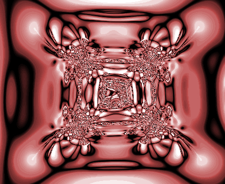
Example. \phi (z,t)=\frac{2t-\cos y}{1-\sin x\cos y}+i\frac{1-2t\sin x}{1-\sin x\cos y}, \int_0^1 \psi (z,t) , dt

Example. Let:

:g_n(z)=z+\frac{c_n}{n}\phi (z), \quad \text{with} \quad f(z) = z + \phi(z).

Next, set T_{1,n}(z)=g_n(z), T_{k,n}(z)= g_n(T_{k-1,n}(z)), and Tn(z) = Tn,n(z). Let

:T(z)=\lim_{n\to \infty} T_n(z)

when that limit exists. The sequence {Tn(z)} defines contours γ = γ(cn, z) that follow the flow of the vector field f(z). If there exists an attractive fixed point α, meaning |f(z) − α| ≤ ρ|z − α| for 0 ≤ ρ n*(z) → T(z) ≡ α along γ = γ(cn, z), provided (for example) c_n = \sqrt{n}. If cn ≡ c 0, then Tn(z) → T(z), a point on the contour γ = γ(c, z). It is easily seen that

:\oint_\gamma \phi (\zeta ) , d\zeta =\lim_{n\to \infty}\frac c n \sum_{k=1}^n \phi ^2 \left (T_{k-1,n}(z) \right )

and

:L(\gamma (z))=\lim_{n\to \infty} \frac{c}{n}\sum_{k=1}^n \left| \phi \left (T_{k-1,n}(z) \right ) \right|,

when these limits exist.

These concepts are marginally related to active contour theory in image processing, and are simple generalizations of the Euler method

Self-replicating expansions

Series

The series defined recursively by fn(z) = z + gn(z) have the property that the nth term is predicated on the sum of the first n − 1 terms. In order to employ theorem (GF3) it is necessary to show boundedness in the following sense: If each fn is defined for |z| n*(z)| n*(z) − z| = |gn(z)| ≤ Cβn is defined for iterative purposes. This is because g_n(G_{n-1}(z)) occurs throughout the expansion. The restriction

:|z|0

serves this purpose. Then Gn(z) → G(z) uniformly on the restricted domain.

Example (S1). Set :f_n(z)=z+\frac{1}{\rho n^2}\sqrt{z}, \qquad \rho \sqrt{\frac{\pi}{6}} and M = ρ2. Then R = ρ2 − (π/6) 0. Then, if S=\left{ z: |z|0 \right}, z in S implies |Gn(z)|

:\begin{align} G_n(z) &=z+g_1(z)+g_2(G_1(z))+g_3(G_2(z))+\cdots + g_n(G_{n-1}(z)) \ &= z+\frac{1}{\rho \cdot 1^2}\sqrt{z}+\frac{1}{\rho \cdot 2^2}\sqrt{G_1(z)}+\frac{1}{\rho \cdot 3^2}\sqrt{G_2(z)}+\cdots +\frac{1}{\rho \cdot n^2} \sqrt{G_{n-1}(z)} \end{align}

converges absolutely, hence is convergent.

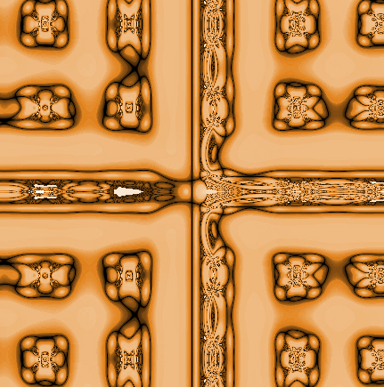
Example (S2): f_n(z)=z+\frac 1 {n^2}\cdot \varphi (z), \varphi (z)=2\cos(x/y)+i2\sin (x/y), G_n(z)=f_n \circ f_{n-1}\circ \cdots \circ f_1(z), \qquad [-10,10], n=50

Products

The product defined recursively by

:f_n(z)=z( 1+g_n(z)), \qquad |z| \leqslant M,

has the appearance

:G_n(z) = z \prod {k=1}^n \left( 1+g_k \left( G{k-1}(z) \right) \right).

In order to apply Theorem GF3 it is required that:

:\left| zg_n(z) \right|\le C\beta_n, \qquad \sum_{k=1}^\infty \beta_k

Once again, a boundedness condition must support

:\left|G_{n-1}(z) g_n(G_{n-1}(z))\right|\le C \beta_n.

If one knows Cβn in advance, the following will suffice:

:|z| \leqslant R = \frac{M}{P} \qquad \text{where} \quad P = \prod_{n=1}^\infty \left( 1+C\beta_n\right).

Then Gn(z) → G(z) uniformly on the restricted domain.

Example (P1). Suppose f_n(z)=z(1+g_n(z)) with g_n(z)=\tfrac{z^2}{n^3}, observing after a few preliminary computations, that |z| ≤ 1/4 implies |Gn(z)|

:\left|G_n(z) \frac{G_n(z)^2}{n^3} \right|

and

:G_n(z)=z \prod_{k=1}^{n-1}\left( 1+\frac{G_k(z)^2}{n^3}\right)

converges uniformly.

Example (P2).

:g_{k,n}(z)=z\left( 1+\frac 1 n \varphi \left (z,\tfrac k n \right ) \right), :G_{n,n}(z)= \left( g_{n,n}\circ g_{n-1,n}\circ \cdots \circ g_{1,n} \right ) (z) = z\prod_{k=1}^n ( 1+P_{k,n}(z)), :P_{k,n}(z)=\frac 1 n \varphi \left (G_{k-1,n}(z),\tfrac{k}{n} \right ), :\prod_{k=1}^{n-1} \left( 1+P_{k,n}(z) \right) = 1+P_{1,n}(z)+P_{2,n}(z)+\cdots + P_{k-1,n}(z) + R_n(z) \sim \int_0^1 \pi (z,t) , dt + 1+R_n(z), :\varphi (z)=x\cos(y)+iy\sin(x), \int_0^1 (z\pi (z,t)-1) ,dt, \qquad [-15,15]:

Continued fractions

Example (CF1): A self-generating continued fraction.

: \begin{align} F_n(z) &= \frac{\rho (z)}{\delta_1+} \frac{\rho (F_1(z))}{\delta_2 +} \frac{\rho (F_2(z))}{\delta_3+} \cdots \frac{\rho (F_{n-1}(z))}{\delta_n}, \ \rho (z) &= \frac{\cos(y)}{\cos (y)+\sin (x)}+i\frac{\sin(x)}{\cos (y)+\sin (x)}, \qquad [0 \end{align}

Example (CF2): Best described as a self-generating reverse Euler continued fraction.

: G_n(z)=\frac{\rho (G_{n-1}(z))}{1+\rho (G_{n-1}(z))-}\ \frac{\rho (G_{n-2}(z))}{1+\rho (G_{n-2}(z))-}\cdots \frac{\rho (G_1(z))}{1+\rho (G_1(z))-}\ \frac{\rho (z)}{1+\rho (z)-z}, :\rho (z)=\rho (x+iy)=x\cos(y)+iy\sin(x), \qquad [-15,15], n=30

References

References

1. Gill, John. (1988). "Compositions of analytic functions of the form Fn(z)=Fn-1(fn(z)),fn->f". Journal of Computational and Applied Mathematics.
2. Henrici, P.. (1988). "Applied and Computational Complex Analysis". Wiley.
3. (November 1990). "Compositions of contractions". Journal of Computational and Applied Mathematics.
4. Gill, J.. (1991). "The use of the sequence F_n(z)=f_n∘⋯∘f₁(z) in computing the fixed points of continued fractions, products, and series". Appl. Numer. Math..
5. (2007). "Accumulation constants of iterated function systems with Bloch target domains.". Finnish Academy of Science and Letters.
6. (2003). "Complex dynamics and related topics: lectures from the Morningside Center of Mathematics". International Press.
7. Gill, J.. (2017). "A Primer on the Elementary Theory of Infinite Compositions of Complex Functions". Communications in the Analytic Theory of Continued Fractions.
8. (May 2012). "On the convergence of infinite compositions of entire functions". Archiv der Mathematik.
9. Gill, J.. (2012). "Convergence of Infinite Compositions of Complex Functions". Communications in the Analytic Theory of Continued Fractions.
10. (1957). "Convergence properties of sequences of linear fractional transformations.". Michigan Mathematical Journal.
11. (December 1962). "On sequences of Moebius transformations". Mathematische Zeitschrift.
12. (1970). "On convergence of sequences of linear fractional transformations". Mathematische Zeitschrift.
13. (1973). "Infinite compositions of Möbius transformations". Transactions of the American Mathematical Society.
14. Steinmetz, N.. (2011). "Rational Iteration". de Gruyter.