From Surf Wiki (app.surf) — the open knowledge base
Gamma distribution
Probability distribution

Probability distribution
| Field | Value | |||
|---|---|---|---|---|
| name | Gamma | |||
| type | density | |||
| pdf_image | [[Image:Gammapdf252.svg | 325px | class=skin-invert-image | Probability density plots of gamma distributions]] |
| cdf_image | [[Image:Gammacdf252.svg | 325px | class=skin-invert-image | Cumulative distribution plots of gamma distributions]] |
| support | x \in 0, \infty) | |||
| f(x)=\frac{1}{\Gamma(\alpha) \theta^\alpha} x^{\alpha - 1} e^{-x/\theta} | ||||
| cdf | F(x)=\frac{1}{\Gamma(\alpha)} \gamma\left(\alpha, \frac{x}{\theta}\right) | |||
| mean | \alpha \theta | |||
| median | Simple closed form does not exist | |||
| mode | (\alpha - 1)\theta \text{ for } \alpha \geq 1, 0 \text{ for } \alpha | |||
| variance | \alpha \theta^2 | |||
| skewness | \frac{2}{\sqrt{\alpha |
- α 0 [shape
- θ 0 scale \alpha &+ \ln\theta + \ln\Gamma(\alpha)\ &+ (1 - \alpha)\psi(\alpha) \end{align} | α 0 shape | λ 0 rate \alpha &- \ln \lambda + \ln\Gamma(\alpha)\ &+ (1 - \alpha)\psi(\alpha) \end{align}
In probability theory and statistics, the gamma distribution is a versatile two-parameter family of continuous probability distributions. The exponential distribution, Erlang distribution, and chi-squared distribution are special cases of the gamma distribution. There are two equivalent parameterizations in common use:
- With a shape parameter α and a scale parameter θ
- With a shape parameter \alpha and a rate parameter In each of these forms, both parameters are positive real numbers.
The distribution has important applications in various fields, including econometrics, Bayesian statistics, and life testing. In econometrics, the (α, θ) parameterization is common for modeling waiting times, such as the time until death, where it often takes the form of an Erlang distribution for integer α values. Bayesian statisticians prefer the (α,λ) parameterization, utilizing the gamma distribution as a conjugate prior for several inverse scale parameters, facilitating analytical tractability in posterior distribution computations.
The gamma distribution is the maximum entropy probability distribution (both with respect to a uniform base measure and a 1/x base measure) for a random variable X for which is fixed and greater than zero, and is fixed (ψ is the digamma function).
Definitions
The parameterization with α and θ appears to be more common in econometrics and other applied fields, where the gamma distribution is frequently used to model waiting times. For instance, in life testing, the waiting time until death is a random variable that is frequently modeled with a gamma distribution. See Hogg and Craig for an explicit motivation.
The parameterization with α and λ is more common in Bayesian statistics, where the gamma distribution is used as a conjugate prior distribution for various types of inverse scale (rate) parameters, such as the λ of an exponential distribution or a Poisson distribution – or for that matter, the λ of the gamma distribution itself. The closely related inverse-gamma distribution is used as a conjugate prior for scale parameters, such as the variance of a normal distribution.
If α is a positive integer, then the distribution represents an Erlang distribution; i.e., the sum of α independent exponentially distributed random variables, each of which has a mean of θ.
Characterization using shape ''α'' and rate ''λ''
The gamma distribution can be parameterized in terms of a shape parameter and an inverse scale parameter , called a rate parameter. A random variable X that is gamma-distributed with shape α and rate λ is denoted
X \sim \Gamma(\alpha, \lambda) \equiv \operatorname{Gamma}(\alpha,\lambda)
The corresponding probability density function in the shape-rate parameterization is
\begin{align} f(x;\alpha,\lambda) & = \frac{ x^{\alpha-1} e^{-\lambda x} \lambda^\alpha}{\Gamma(\alpha)} \quad \text{ for } x 0 \quad \alpha, \lambda 0, \[6pt] \end{align}
where \Gamma(\alpha) is the gamma function. For all positive integers, \Gamma(\alpha)=(\alpha-1)!.
The cumulative distribution function is the regularized gamma function:
F(x;\alpha,\lambda) = \int_0^x f(u;\alpha,\lambda),du= \frac{\gamma(\alpha, \lambda x)}{\Gamma(\alpha)},
where \gamma(\alpha, \lambda x) is the lower incomplete gamma function.
If α is a positive integer (i.e., the distribution is an Erlang distribution), the cumulative distribution function has the following series expansion:
\begin{align} F(x;\alpha,\lambda) &= 1-\sum_{i=0}^{\alpha-1} \frac{\left(\lambda x\right)^i}{i!} e^{-\lambda x} \[1ex] &= e^{-\lambda x} \sum_{i=\alpha}^\infty \frac{\left(\lambda x\right)^i}{i!}. \end{align}
Characterization using shape ''α'' and scale ''θ''
A random variable X that is gamma-distributed with shape α and scale θ is denoted by
X \sim \Gamma(\alpha, \theta) \equiv \operatorname{Gamma}(\alpha, \theta)
The probability density function using the shape-scale parametrization is
f(x;\alpha,\theta) = \frac{x^{\alpha-1}e^{-x/\theta}}{\theta^\alpha\Gamma(\alpha)} \quad \text{ for } x 0 \text{ and } \alpha, \theta 0.
Here Γ(α) is the gamma function evaluated at α.
The cumulative distribution function is the regularized gamma function:
F(x;\alpha,\theta) = \int_0^x f(u;\alpha,\theta),du = \frac{\gamma{\left(\alpha, \frac{x}{\theta}\right)}}{\Gamma(\alpha)},
where \gamma{\left(\alpha, \frac{x}{\theta}\right)} is the lower incomplete gamma function.
It can also be expressed as follows, if α is a positive integer (i.e., the distribution is an Erlang distribution):
F(x;\alpha,\theta) = 1-\sum_{i=0}^{\alpha-1} \frac{1}{i!} \left(\frac{x}{\theta} \right)^i e^{-x/\theta} = e^{-x/\theta} \sum_{i=\alpha}^\infty \frac{1}{i!} \left( \frac{x}{\theta} \right)^i.
Both parametrizations are common because either can be more convenient depending on the situation.
Properties
Mean and variance
The mean of gamma distribution is given by the product of its shape and scale parameters: \mu = \alpha\theta = \alpha/\lambda The variance is: \sigma^2 = \alpha \theta^2 = \alpha/\lambda^2 The square root of the inverse shape parameter gives the coefficient of variation: \sigma/\mu = \alpha^{-0.5} = 1/\sqrt{\alpha}
Skewness
The skewness of the gamma distribution only depends on its shape parameter, α, and it is equal to 2/\sqrt{\alpha}.
Higher moments
The r-th raw moment is given by: : \mathrm{E}[X^r] = \theta^r \frac{\Gamma(\alpha+r)}{\Gamma(\alpha)} = \theta^r \alpha^\overline{r} with \alpha^\overline{r} the rising factorial.
Median approximations and bounds
Unlike the mode and the mean, which have readily calculable formulas based on the parameters, the median does not have a closed-form equation. The median for this distribution is the value \nu such that \frac{1}{\Gamma(\alpha) \theta^\alpha} \int_0^{\nu} x^{\alpha - 1} e^{-x/\theta} dx = \frac{1}{2}.
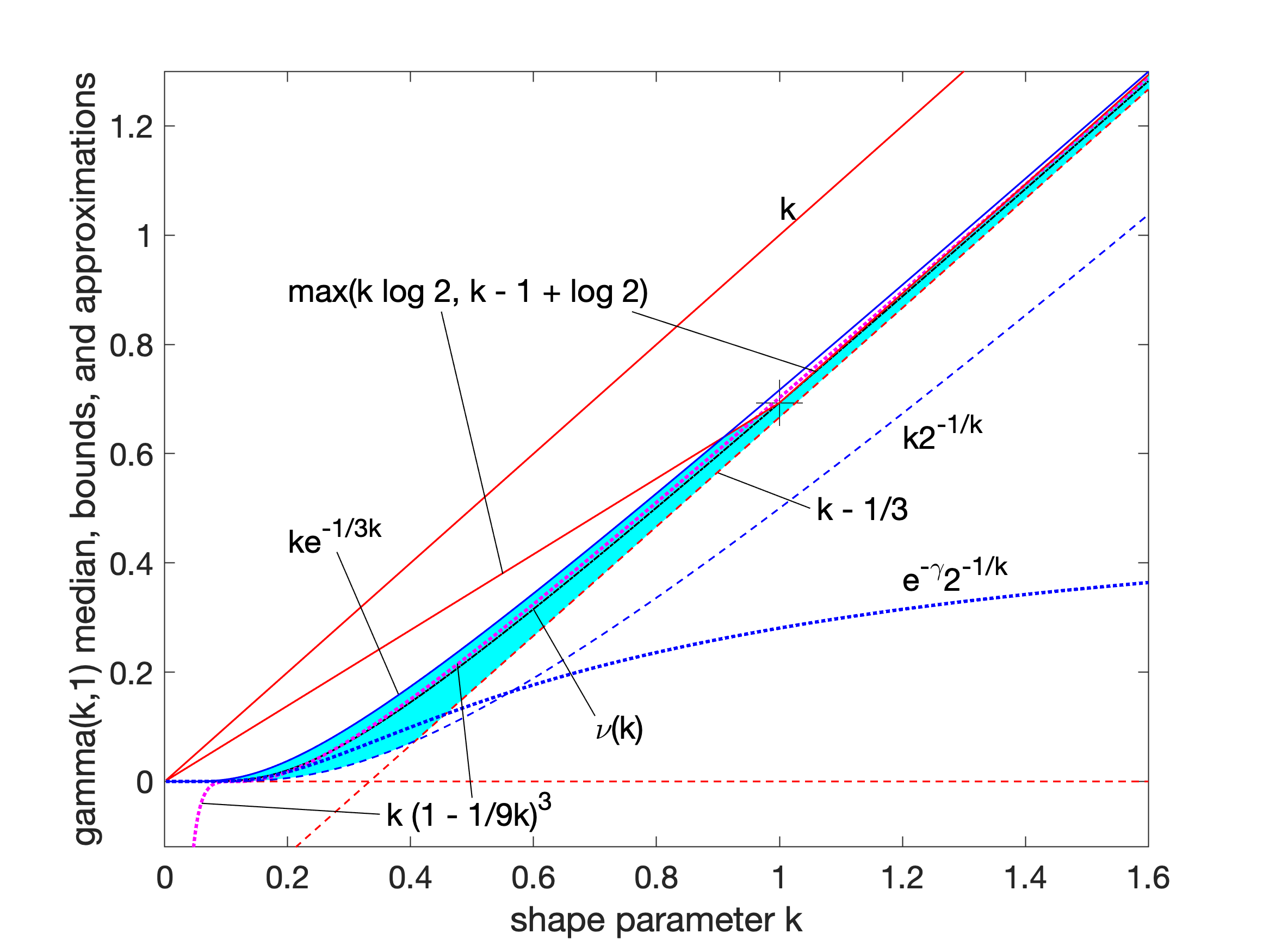
A rigorous treatment of the problem of determining an asymptotic expansion and bounds for the median of the gamma distribution was handled first by Chen and Rubin, who proved that (for \theta = 1) \alpha - \tfrac{1}{3} where \mu(\alpha) = \alpha is the mean and \nu(\alpha) is the median of the \text{Gamma}(\alpha,1) distribution. For other values of the scale parameter, the mean scales to \mu = \alpha\theta, and the median bounds and approximations would be similarly scaled by θ.
K. P. Choi found the first five terms in a Laurent series asymptotic approximation of the median by comparing the median to Ramanujan's \theta function. Berg and Pedersen found more terms: \begin{align} \nu(\alpha) = \alpha & - \frac{1}{3} + \frac{8}{405} \alpha^{-1} + \frac{184} \alpha^{-2} + \frac{2248} \alpha^{-3} \[1ex] & - \frac{19,006,408} \alpha^{-4} - \mathcal{O}{\left(\alpha^{-5}\right)} + \cdots \end{align}

Partial sums of these series are good approximations for high enough α; they are not plotted in the figure, which is focused on the low-α region that is less well approximated.
Berg and Pedersen also proved many properties of the median, showing that it is a convex function of α, and that the asymptotic behavior near \alpha = 0 is \nu(\alpha) \approx e^{-\gamma}2^{-1/\alpha} (where γ is the Euler–Mascheroni constant), and that for all \alpha 0 the median is bounded by \alpha 2^{-1/\alpha} .
A closer linear upper bound, for \alpha \ge 1 only, was provided in 2021 by Gaunt and Merkle, relying on the Berg and Pedersen result that the slope of \nu(\alpha) is everywhere less than 1: \nu(\alpha) \le \alpha - 1 + \log2 ~~ for \alpha \ge 1 (with equality at \alpha = 1) which can be extended to a bound for all \alpha 0 by taking the max with the chord shown in the figure, since the median was proved convex.
An approximation to the median that is asymptotically accurate at high α and reasonable down to \alpha = 0.5 or a bit lower follows from the Wilson–Hilferty transformation: \nu(\alpha) = \alpha \left( 1 - \frac{1}{9\alpha} \right)^3 which goes negative for \alpha .
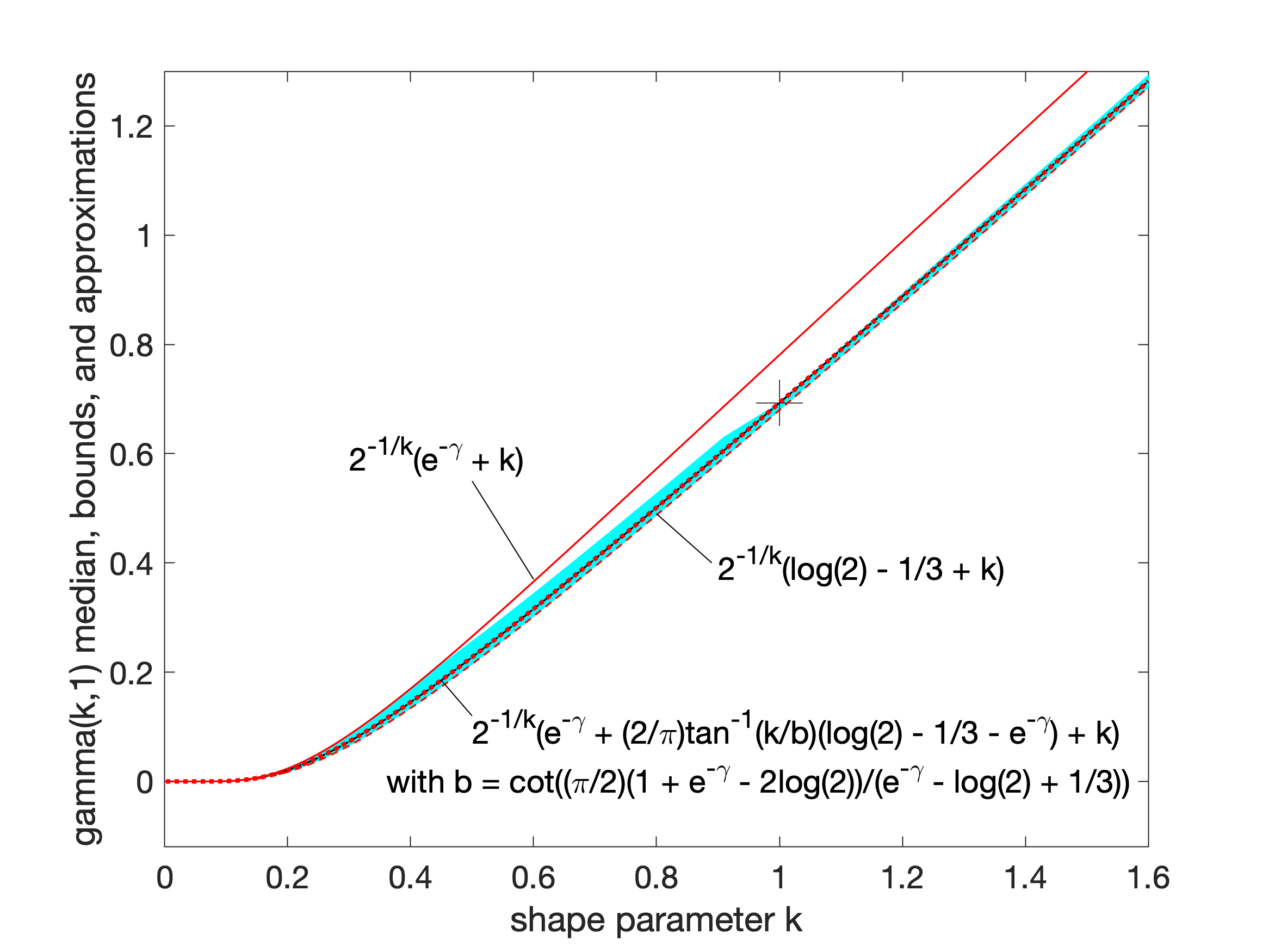
In 2021, Lyon proposed several approximations of the form \nu(\alpha) \approx 2^{-1/\alpha}(A + B\alpha). He conjectured values of A and B for which this approximation is an asymptotically tight upper or lower bound for all \alpha 0. In particular, he proposed these closed-form bounds, which he proved in 2023:
\nu_{L\infty}(\alpha) = 2^{-1/\alpha} \left(\log 2 - \tfrac{1}{3} + \alpha\right) is a lower bound, asymptotically tight as \alpha \to \infty \nu_U(\alpha) = 2^{-1/\alpha}(e^{-\gamma} + \alpha) \quad is an upper bound, asymptotically tight as \alpha \to 0
Lyon also showed (informally in 2021, rigorously in 2023) two other lower bounds that are not closed-form expressions, including this one involving the gamma function, based on solving the integral expression substituting 1 for e^{-x}: \nu(\alpha) \left( \frac{2}{\Gamma(\alpha+1)} \right)^{-1/\alpha} (approaching equality as k \to 0) and the tangent line at \alpha = 1 where the derivative was found to be \nu^\prime(1) \approx 0.9680448: \nu(\alpha) \ge \nu(1) + (\alpha-1) \nu^\prime(1) \quad (with equality at k = 1) \nu(\alpha) \ge \log 2 + (\alpha-1) \left[\gamma - 2 \operatorname{Ei}(-\log 2) - \log \log 2\right] where Ei is the exponential integral.
Additionally, he showed that interpolations between bounds could provide excellent approximations or tighter bounds to the median, including an approximation that is exact at \alpha = 1 (where \nu(1) = \log 2) and has a maximum relative error less than 0.6%. Interpolated approximations and bounds are all of the form \nu(\alpha) \approx \tilde{g}(\alpha)\nu_{L\infty}(\alpha) + (1 - \tilde{g}(\alpha)) \nu_U(\alpha) where \tilde{g} is an interpolating function running monotonially from 0 at low α to 1 at high α, approximating an ideal, or exact, interpolator g(\alpha): g(\alpha) = \frac{\nu_U(\alpha) - \nu(\alpha)}{\nu_U(\alpha) - \nu_{L\infty}(\alpha)} For the simplest interpolating function considered, a first-order rational function \tilde{g}_1(\alpha) = \frac{\alpha}{b_0 + \alpha} the tightest lower bound has b_0 = \frac{\frac{8}{405} + e^{-\gamma} \log 2 - \frac{\log^2 2}{2}}{e^{-\gamma} - \log 2 + \frac{1}{3}} - \log 2 \approx 0.143472 and the tightest upper bound has b_0 = \frac{e^{-\gamma} - \log 2 + \frac{1}{3}}{1 - \frac{e^{-\gamma} \pi^2}{12}} \approx 0.374654 The interpolated bounds are plotted (mostly inside the yellow region) in the log–log plot shown. Even tighter bounds are available using different interpolating functions, but not usually with closed-form parameters like these.
Summation
If X**i has a Gamma(α**i, θ) distribution for (i.e., all distributions have the same scale parameter θ), then
\sum_{i=1}^N X_i \sim\mathrm{Gamma} \left( \sum_{i=1}^N \alpha_i, \theta \right)
provided all X**i are independent.
For the cases where the X**i are independent but have different scale parameters, see Mathai or Moschopoulos.
The gamma distribution exhibits infinite divisibility.
Scaling
If X \sim \mathrm{Gamma}(\alpha, \theta),
then, for any c 0,
cX \sim \mathrm{Gamma}(\alpha, c,\theta), by moment generating functions,
or equivalently, if
X \sim \mathrm{Gamma}\left( \alpha,\lambda \right) (shape-rate parameterization)
cX \sim \mathrm{Gamma}\left( \alpha, \frac \lambda c \right),
Indeed, we know that if X is an exponential r.v. with rate λ, then cX is an exponential r.v. with rate λ/c; the same thing is valid with Gamma variates (and this can be checked using the moment-generating function, see, e.g.,these notes, 10.4-(ii)): multiplication by a positive constant c divides the rate (or, equivalently, multiplies the scale).
Exponential family
The gamma distribution is a two-parameter exponential family with natural parameters α − 1 and −1/θ (equivalently, α − 1 and −λ), and natural statistics X and ln X.
If the shape parameter α is held fixed, the resulting one-parameter family of distributions is a natural exponential family.
Logarithmic expectation and variance
One can show that
\operatorname{E}[\ln X] = \psi(\alpha) - \ln \lambda
or equivalently,
\operatorname{E}[\ln X] = \psi(\alpha) + \ln \theta
where ψ is the digamma function. Likewise,
\operatorname{var}[\ln X] = \psi^{(1)}(\alpha)
where \psi^{(1)} is the trigamma function.
This can be derived using the exponential family formula for the moment generating function of the sufficient statistic, because one of the sufficient statistics of the gamma distribution is ln x.
Information entropy
The information entropy is
\begin{align} \operatorname{H}(X) & = \operatorname{E}[-\ln p(X)] \[4pt] & = \operatorname{E}[-\alpha \ln \lambda + \ln \Gamma(\alpha) - (\alpha-1)\ln X + \lambda X] \[4pt] & = \alpha - \ln \lambda + \ln \Gamma(\alpha) + (1-\alpha)\psi(\alpha). \end{align}
In the α, θ parameterization, the information entropy is given by
\operatorname{H}(X) =\alpha + \ln \theta + \ln \Gamma(\alpha) + (1-\alpha)\psi(\alpha).
Kullback–Leibler divergence

The Kullback–Leibler divergence (KL-divergence), of Gamma(α**p, λ**p) ("true" distribution) from Gamma(α**q, λ**q) ("approximating" distribution) is given by
\begin{align} D_{\mathrm{KL}}(\alpha_p,\lambda_p; \alpha_q, \lambda_q) = {} & (\alpha_p-\alpha_q) \psi(\alpha_p) - \log\frac{\Gamma(\alpha_p)}{\Gamma(\alpha_q)} \ & {} + \alpha_q \log\frac{\lambda_p}{\lambda_q} + \alpha_p\left(\frac{\lambda_q}{\lambda_p} - 1\right). \end{align}
Written using the α, θ parameterization, the KL-divergence of Gamma(α**p, θ**p) from Gamma(α**q, θ**q) is given by
\begin{align} D_{\mathrm{KL}}(\alpha_p,\theta_p; \alpha_q, \theta_q) = {} & (\alpha_p-\alpha_q)\psi(\alpha_p) - \log\frac{\Gamma(\alpha_p)}{\Gamma(\alpha_q)} \ & {} + \alpha_q \log\frac{\theta_q}{\theta_p} + \alpha_p \left(\frac{\theta_p}{\theta_q} - 1 \right). \end{align}
Laplace transform
The Laplace transform of the gamma PDF, which is the moment-generating function of the gamma distribution, is
F(s) = \operatorname E\left[ e^{-sX} \right] = \frac{1}{\left(1 + \theta s\right)^\alpha} = \left( \frac\lambda{ \lambda + s} \right)^\alpha
(where X is a random variable with that distribution).
Statistical inference
Parameter estimation
Maximum likelihood estimation
The likelihood function for N iid observations (x1, ..., x**N) is
L(\alpha, \theta) = \prod_{i=1}^N f(x_i;\alpha,\theta)
from which we calculate the log-likelihood function
\ell(\alpha, \theta) = (\alpha - 1) \sum_{i=1}^N \ln x_i - \sum_{i=1}^N \frac{x_i} \theta - N\alpha\ln \theta - N\ln \Gamma(\alpha)
Finding the maximum with respect to θ by taking the derivative and setting it equal to zero yields the maximum likelihood estimator of the θ parameter, which equals the sample mean \bar{x} divided by the shape parameter α:
\hat{\theta} = \frac{1}{\alpha N}\sum_{i=1}^N x_i = \frac{\bar{x}}{\alpha}
Substituting this into the log-likelihood function gives
\ell(\alpha) = (\alpha-1)\sum_{i=1}^N \ln x_i -N\alpha - N\alpha\ln \frac{\sum_i x_i}{\alpha N} - N\ln \Gamma(\alpha)
We need at least two samples: N\ge2, because for N=1, the function \ell(\alpha) increases without bounds as \alpha\to\infty. For \alpha0, it can be verified that \ell(\alpha) is strictly concave, by using inequality properties of the polygamma function. Finding the maximum with respect to α by taking the derivative and setting it equal to zero yields
\begin{align} \ln \alpha - \psi(\alpha) &= \ln\left(\frac{1}{N}\sum_{i=1}^N x_i\right) - \frac 1 N \sum_{i=1}^N \ln x_i \[1ex] &= \ln \bar{x} - \overline{\ln x} \end{align}
where ψ is the digamma function and \overline{\ln x} is the sample mean of ln x. There is no closed-form solution for α. The function is numerically very well behaved, so if a numerical solution is desired, it can be found using, for example, Newton's method. An initial value of k can be found either using the method of moments, or using the approximation
\ln \alpha - \psi(\alpha) \approx \frac{1}{2\alpha}\left(1 + \frac{1}{6\alpha + 1} \right)
If we let
\begin{align} s &= \ln \left(\frac 1 N \sum_{i=1}^N x_i\right) - \frac 1 N \sum_{i=1}^N \ln x_i \[1ex] &= \ln \bar{x} - \overline{\ln x} \end{align}
then α is approximately
k \approx \frac{3 - s + \sqrt{\left(s - 3\right)^2 + 24s}}{12s}
which is within 1.5% of the correct value. An explicit form for the Newton–Raphson update of this initial guess is:
\alpha \leftarrow \alpha - \frac{ \ln \alpha - \psi(k) - s }{ \frac 1 \alpha - \psi\prime(\alpha) }.
At the maximum-likelihood estimate (\hat \alpha,\hat\theta), the expected values for x and \ln x agree with the empirical averages: \begin{align} \hat \alpha\hat\theta &= \bar x &&\text{and} & \psi(\hat \alpha)+\ln \hat\theta &= \overline{\ln x}. \end{align}
Caveat for small shape parameter
For data, (x_1,\ldots,x_N), that is represented in a floating point format that underflows to 0 for values smaller than \varepsilon, the logarithms that are needed for the maximum-likelihood estimate will cause failure if there are any underflows. If we assume the data was generated by a gamma distribution with cdf F(x;\alpha,\theta), then the probability that there is at least one underflow is: \Pr(\text{underflow}) = 1-(1-F(\varepsilon;\alpha,\theta))^N This probability will approach 1 for small α and large N. For example, at \alpha=10^{-2}, N=10^4 and \varepsilon=2.25\times10^{-308}, \Pr(\text{underflow})\approx 0.9998. A workaround is to instead have the data in logarithmic format.
In order to test an implementation of a maximum-likelihood estimator that takes logarithmic data as input, it is useful to be able to generate non-underflowing logarithms of random gamma variates, when \alpha. Following the implementation in scipy.stats.loggamma, this can be done as follows: sample Y\sim\text{Gamma}(\alpha+1,\theta) and U\sim\text{Uniform} independently. Then the required logarithmic sample is Z=\ln(Y)+\ln(U)/\alpha, so that \exp(Z)\sim\text{Gamma}(k,\theta).
Closed-form estimators
There exist consistent closed-form estimators of α and θ that are derived from the likelihood of the generalized gamma distribution.
The estimate for the shape α is
\hat{\alpha} = \frac{N \sum\limits_{i=1}^N x_i}{N \sum\limits_{i=1}^N x_i \ln x_i - \sum\limits_{i=1}^N x_i \sum\limits_{i=1}^N \ln x_i}
and the estimate for the scale θ is
\hat{\theta} = \frac{1}{N^2} \left(N \sum_{i=1}^N x_i \ln x_i - \sum_{i=1}^N x_i \sum_{i=1}^N \ln x_i\right)
Using the sample mean of x, the sample mean of ln x, and the sample mean of the product x·ln x simplifies the expressions to:
\hat{\alpha} = \frac{\bar{x}}{\hat{\theta}} \hat{\theta} = \overline{x\ln x} - \bar{x} \overline{\ln x}.
If the rate parameterization is used, the estimate of \hat{\lambda} = 1/\hat{\theta}.
These estimators are not strictly maximum likelihood estimators, but are instead referred to as mixed type log-moment estimators. They have however similar efficiency as the maximum likelihood estimators.
Although these estimators are consistent, they have a small bias. A bias-corrected variant of the estimator for the scale θ is
\tilde{\theta} = \frac{N}{N - 1} \hat{\theta}
A bias correction for the shape parameter α is given as
\tilde{\alpha} = \hat{\alpha} - \frac{1}{N} \left(3 \hat{\alpha} - \frac{2}{3} \left(\frac{\hat{\alpha}}{1 + \hat{\alpha}}\right) - \frac{4}{5} \frac{\hat{\alpha}}{(1 + \hat{\alpha})^2} \right)
Bayesian minimum mean squared error
With known α and unknown θ, the posterior density function for theta (using the standard scale-invariant prior for θ) is
\Pr(\theta \mid \alpha, x_1, \dots, x_N) \propto \frac 1 \theta \prod_{i=1}^N f(x_i; \alpha, \theta)
Denoting
y \equiv \sum_{i=1}^Nx_i , \qquad \Pr(\theta \mid \alpha, x_1, \dots, x_N) = C(x_i) \theta^{-N \alpha-1} e^{-y/\theta}
where the C (integration) constant does not depend on θ. The form of the posterior density reveals that 1 / θ is gamma-distributed with shape parameter Nα + 2 and rate parameter y. Integration with respect to θ can be carried out using a change of variables to find the integration constant
\begin{align} \int_0^\infty \theta^{-N\alpha - 1 + m} e^{-y/\theta}, d\theta &= \int_0^\infty x^{N\alpha - 1 - m} e^{-xy} , dx \ &= y^{-(N\alpha - m)} \Gamma(N\alpha - m) ! \end{align}
The moments can be computed by taking the ratio (m by )
\operatorname{E} [x^m] = \frac {\Gamma (N\alpha - m)} {\Gamma(N\alpha)} y^m
which shows that the mean ± standard deviation estimate of the posterior distribution for θ is
\frac y {N\alpha - 1} \pm \sqrt{\frac {y^2} {\left(N\alpha - 1\right)^2 (N\alpha - 2)}}.
Bayesian inference
Conjugate prior
In Bayesian inference, the gamma distribution is the conjugate prior to many likelihood distributions: the Poisson, exponential, normal (with known mean), Pareto, gamma with known shape σ, inverse gamma with known shape parameter, and Gompertz with known scale parameter.
The gamma distribution's conjugate prior is:
p(\alpha,\theta \mid p, q, r, s) = \frac{1}{Z} \frac{p^{\alpha-1} e^{-\theta^{-1} q}}{\Gamma(\alpha)^r \theta^{\alpha s}},
where Z is the normalizing constant with no closed-form solution. The posterior distribution can be found by updating the parameters as follows:
\begin{align} p' &= p\prod\nolimits_i x_i,\ q' &= q + \sum\nolimits_i x_i,\ r' &= r + n,\ s' &= s + n, \end{align}
where n is the number of observations, and x**i is the i-th observation from the gamma distribution.
Occurrence and applications
Consider a sequence of events, with the waiting time for each event being an exponential distribution with rate λ. Then the waiting time for the n-th event to occur is the gamma distribution with integer shape \alpha = n. This construction of the gamma distribution allows it to model a wide variety of phenomena where several sub-events, each taking time with exponential distribution, must happen in sequence for a major event to occur. Examples include the waiting time of cell-division events, number of compensatory mutations for a given mutation, waiting time until a repair is necessary for a hydraulic system, and so on.
In biophysics, the dwell time between steps of a molecular motor like ATP synthase is nearly exponential at constant ATP concentration, revealing that each step of the motor takes a single ATP hydrolysis. If there were n ATP hydrolysis events, then it would be a gamma distribution with degree n.
The gamma distribution has been used to model the size of insurance claims and rainfalls. This means that aggregate insurance claims and the amount of rainfall accumulated in a reservoir are modelled by a gamma process – much like the exponential distribution generates a Poisson process.
The gamma distribution is also used to model errors in multi-level Poisson regression models because a mixture of Poisson distributions with gamma-distributed rates has a known closed form distribution, called negative binomial.
In wireless communication, the gamma distribution is used to model the multi-path fading of signal power; see also Rayleigh distribution and Rician distribution.
In oncology, the age distribution of cancer incidence often follows the gamma distribution, wherein the shape and scale parameters predict, respectively, the number of driver events and the time interval between them.
In neuroscience, the gamma distribution is often used to describe the distribution of inter-spike intervals.
In bacterial gene expression where protein production can occur in bursts, the copy number of a given protein often follows the gamma distribution, where the shape and scale parameters are, respectively, the mean number of bursts per cell cycle and the mean number of protein molecules produced per burst.
In genomics, the gamma distribution was applied in peak calling step (i.e., in recognition of signal) in ChIP-chip and ChIP-seq data analysis.
In Bayesian statistics, the gamma distribution is widely used as a conjugate prior. It is the conjugate prior for the precision (i.e. inverse of the variance) of a normal distribution. It is also the conjugate prior for the exponential distribution.
In phylogenetics, the gamma distribution is the most commonly used approach to model among-sites rate variation when maximum likelihood, Bayesian, or distance matrix methods are used to estimate phylogenetic trees. Phylogenetic analyzes that use the gamma distribution to model rate variation estimate a single parameter from the data because they limit consideration to distributions where . This parameterization means that the mean of this distribution is 1 and the variance is 1/α. Maximum likelihood and Bayesian methods typically use a discrete approximation to the continuous gamma distribution.
Random variate generation
Given the scaling property above, it is enough to generate gamma variables with , as we can later convert to any value of λ with a simple division.
Suppose we wish to generate random variables from Gamma(n + δ, 1), where n is a non-negative integer and {{math|0
-\sum_{k=1}^n \ln U_k \sim \Gamma(n, 1)
where U**k are all uniformly distributed on (0, 1] and independent. All that is left now is to generate a variable distributed as Gamma(δ, 1) for {{math|0
Random generation of gamma variates is discussed in detail by Devroye, noting that none are uniformly fast for all shape parameters. For small values of the shape parameter, the algorithms are often not valid. For arbitrary values of the shape parameter, one can apply the Ahrens and Dieter modified acceptance-rejection method Algorithm GD (shape α ≥ 1), or transformation method when {{math|0
The following is a version of the Ahrens-Dieter acceptance–rejection method:
- Generate U, V and W as iid uniform (0, 1] variates.
- If U\le\frac e {e+\delta} then \xi=V^{1/\delta} and \eta=W\xi^{\delta-1}. Otherwise, \xi=1-\ln V and \eta=We^{-\xi}.
- If \eta\xi^{\delta-1}e^{-\xi} then go to step 1.
- ξ is distributed as Γ(δ, 1).
A summary of this is \theta \left( \xi - \sum_{i=1}^{\lfloor \alpha \rfloor} \ln U_i \right) \sim \Gamma (\alpha, \theta) where \scriptstyle \lfloor \alpha \rfloor is the integer part of α, ξ is generated via the algorithm above with (the fractional part of α) and the U**k are all independent.
While the above approach is technically correct, Devroye notes that it is linear in the value of α and generally is not a good choice. Instead, he recommends using either rejection-based or table-based methods, depending on context.
For example, Marsaglia's simple transformation-rejection method relying on one normal variate X and one uniform variate U:
- Set d = a - \frac13 and c = \frac1{\sqrt{9d}}.
- Set v=(1+cX)^3.
- If v 0 and \ln U return dv, else go back to step 2.
With 1 \le a = \alpha generates a gamma distributed random number in time that is approximately constant with α. The acceptance rate does depend on α, with an acceptance rate of 0.95, 0.98, and 0.99 for α = 1, 2, and 4. For {{math|α \gamma_\alpha = \gamma_{1+\alpha} U^{1/\alpha} to boost k to be usable with this method.
In Matlab numbers can be generated using the function gamrnd(), which uses the α, θ representation.
References
References
- "Gamma distribution {{!}} Probability, Statistics, Distribution {{!}} Britannica".
- Weisstein, Eric W.. "Gamma Distribution".
- "Gamma Distribution {{!}} Gamma Function {{!}} Properties {{!}} PDF".
- (2009). "Maximum entropy autoregressive conditional heteroskedasticity model". Journal of Econometrics.
- (1978). "Introduction to Mathematical Statistics". Macmillan.
- (2013). "Scalable Recommendation with Poisson Factorization".
- Papoulis, Pillai, ''Probability, Random Variables, and Stochastic Processes'', Fourth Edition
- Jeesen Chen, [[Herman Rubin]], Bounds for the difference between median and mean of gamma and Poisson distributions, Statistics & Probability Letters, Volume 4, Issue 6, October 1986, Pages 281–283, {{issn. 0167-7152, [https://dx.doi.org/10.1016/0167-7152(86)90044-1] {{Webarchive. link. (2024-10-09.)
- Choi, K. P. [https://www.ams.org/journals/proc/1994-121-01/S0002-9939-1994-1195477-8/S0002-9939-1994-1195477-8.pdf "On the Medians of the Gamma Distributions and an Equation of Ramanujan"] {{Webarchive. link. (2021-01-23 , Proceedings of the American Mathematical Society, Vol. 121, No. 1 (May, 1994), pp. 245–251.)
- Berg, Christian. (March 2006). "The Chen–Rubin conjecture in a continuous setting". Methods and Applications of Analysis.
- Berg, Christian and Pedersen, Henrik L. [https://arxiv.org/abs/math/0609442 "Convexity of the median in the gamma distribution"] {{Webarchive. link. (2023-05-26 .)
- (2021). "On bounds for the mode and median of the generalized hyperbolic and related distributions". Journal of Mathematical Analysis and Applications.
- (13 May 2021). "On closed-form tight bounds and approximations for the median of a gamma distribution". [[PLOS One]].
- (13 May 2021). "Tight bounds for the median of a gamma distribution". [[PLOS One]].
- Mathai, A. M.. (1982). "Storage capacity of a dam with gamma type inputs". Annals of the Institute of Statistical Mathematics.
- Moschopoulos, P. G.. (1985). "The distribution of the sum of independent gamma random variables". Annals of the Institute of Statistical Mathematics.
- Penny, W. D.. "KL-Divergences of Normal, Gamma, Dirichlet, and Wishart densities".
- "LogGammaDistribution—Wolfram Language Documentation".
- "ExpGammaDistribution—Wolfram Language Documentation".
- "scipy.stats.loggamma — SciPy v1.8.0 Manual".
- (22 June 2021). "The Modified-Half-Normal distribution: Properties and an efficient sampling scheme". Communications in Statistics - Theory and Methods.
- Dubey, Satya D.. (December 1970). "Compound gamma, beta and F distributions". Metrika.
- Minka, Thomas P.. (2002). "Estimating a Gamma distribution".
- (1969). "Maximum Likelihood Estimation of the Parameters of the Gamma Distribution and Their Bias". Technometrics.
- (2017). "Closed-Form Estimators for the Gamma Distribution Derived from Likelihood Equations". The American Statistician.
- (2019). "A Note on Bias of Closed-Form Estimators for the Gamma Distribution Derived from Likelihood Equations". The American Statistician.
- Fink, D. 1995 [http://citeseerx.ist.psu.edu/viewdoc/download?doi=10.1.1.157.5540&rep=rep1&type=pdf A Compendium of Conjugate Priors]. In progress report: Extension and enhancement of methods for setting data quality objectives. (DOE contract 95‑831).
- Jessica., Scheiner, Samuel M., 1956- Gurevitch. (2001). "Design and analysis of ecological experiments". Oxford University Press.
- Golubev, A.. (March 2016). "Applications and implications of the exponentially modified gamma distribution as a model for time variabilities related to cell proliferation and gene expression". Journal of Theoretical Biology.
- (2005-07-01). "The Coupon Collector and the Suppressor Mutation". Genetics.
- (July 1999). "Failure rate distributions for flexible manufacturing systems: An empirical study". European Journal of Operational Research.
- (2000-08-15). "Myosin-V stepping kinetics: A molecular model for processivity". Proceedings of the National Academy of Sciences.
- p. 43, Philip J. Boland, Statistical and Probabilistic Methods in Actuarial Science, Chapman & Hall CRC 2007
- Wilks, Daniel S.. (1990). "Maximum Likelihood Estimation for the Gamma Distribution Using Data Containing Zeros". Journal of Climate.
- (22 September 2017). "The number of key carcinogenic events can be predicted from cancer incidence". Scientific Reports.
- (2021-08-06). "The Erlang distribution approximates the age distribution of incidence of childhood and young adulthood cancers". PeerJ.
- J. G. Robson and J. B. Troy, "Nature of the maintained discharge of Q, X, and Y retinal ganglion cells of the cat", J. Opt. Soc. Am. A 4, 2301–2307 (1987)
- M.C.M. Wright, I.M. Winter, J.J. Forster, S. Bleeck "Response to best-frequency tone bursts in the ventral cochlear nucleus is governed by ordered inter-spike interval statistics", Hearing Research 317 (2014)
- N. Friedman, L. Cai and X. S. Xie (2006) "Linking stochastic dynamics to population distribution: An analytical framework of gene expression", ''Phys. Rev. Lett.'' 97, 168302.
- DJ Reiss, MT Facciotti and NS Baliga (2008) [https://web.archive.org/web/20121117144623/http://bioinformatics.oxfordjournals.org/content/24/3/396.full.pdf+html "Model-based deconvolution of genome-wide DNA binding"], ''Bioinformatics'', 24, 396–403
- MA Mendoza-Parra, M Nowicka, W Van Gool, H Gronemeyer (2013) [http://www.biomedcentral.com/1471-2164/14/834 "Characterising ChIP-seq binding patterns by model-based peak shape deconvolution"] {{Webarchive. link. (2024-10-09 , ''BMC Genomics'', 14:834)
- Yang, Ziheng. (September 1996). "Among-site rate variation and its impact on phylogenetic analyses". Trends in Ecology & Evolution.
- Yang, Ziheng. (September 1994). "Maximum likelihood phylogenetic estimation from DNA sequences with variable rates over sites: Approximate methods". Journal of Molecular Evolution.
- Felsenstein, Joseph. (2001-10-01). "Taking Variation of Evolutionary Rates Between Sites into Account in Inferring Phylogenies". Journal of Molecular Evolution.
- Devroye, Luc. (1986). "Non-Uniform Random Variate Generation". Springer-Verlag.
- (January 1982). "Generating gamma variates by a modified rejection technique". Communications of the ACM.
- (1974). "Computer methods for sampling from gamma, beta, Poisson and binomial distributions". Computing.
- (1979). "Some Simple Gamma Variate Generators". Journal of the Royal Statistical Society. Series C (Applied Statistics).
- Marsaglia, G. The squeeze method for generating gamma variates. Comput, Math. Appl. 3 (1977), 321–325.
- (2000). "A simple method for generating gamma variables". ACM Transactions on Mathematical Software.
This article was imported from Wikipedia and is available under the Creative Commons Attribution-ShareAlike 4.0 License. Content has been adapted to SurfDoc format. Original contributors can be found on the article history page.
Ask Mako anything about Gamma distribution — get instant answers, deeper analysis, and related topics.
Research with MakoFree with your Surf account
Create a free account to save articles, ask Mako questions, and organize your research.
Sign up freeThis content may have been generated or modified by AI. CloudSurf Software LLC is not responsible for the accuracy, completeness, or reliability of AI-generated content. Always verify important information from primary sources.
Report