One-dimensional ESPRIT

At instance t , the M (complex-valued) output signals (measurements) y_m[t], m = 1, \ldots, M , of the system are related to the K (complex-valued) input signals x_k[t] , k = 1, \ldots, K , asy_m[t] = \sum_{k=1}^K a_{m,k} x_k[t] + n_m[t], where n_m[t] denotes the noise added by the system. The one-dimensional form of ESPRIT can be applied if the weights have the form a_{m,k} = e^{-j(m-1)\omega_k} , whose phases are integer multiples of some radial frequency \omega_k . This frequency only depends on the index of the system's input, i.e. k . The goal of ESPRIT is to estimate \omega_k 's, given the outputs y_m[t] and the number of input signals, K . Since the radial frequencies are the actual objectives, a_{m,k} is denoted as a_m(\omega_k) .

Collating the weights a_m(\omega_k) as \mathbf a(\omega_k) = [,1 ,\ e^{-j\omega_k} ,\ e^{-j2\omega_k} ,\ ... ,\ e^{-j(M-1)\omega_k},]^\top and the M output signals at instance t as \mathbf y[t] = [,y_1[t],\ y_2[t] ,\ ... ,\ y_M[t],]^\top, \mathbf y[t] = \sum_{k=1}^K \mathbf a(\omega_k) x_k[t] + \mathbf{n}[t],where \mathbf n[t] = [,n_1[t],\ n_2[t] ,\ ... ,\ n_M[t],]^\top. Further, when the weight vectors \mathbf a(\omega_1), \ \mathbf a(\omega_2),\ ..., \ \mathbf a(\omega_K) are put into a Vandermonde matrix \mathbf A = [,\mathbf a(\omega_1) ,\ \mathbf a(\omega_2) ,\ ... ,\ \mathbf a(\omega_K),], and the K inputs at instance t into a vector \mathbf x[t] = [,x_1[t] ,\ ... ,\ x_K[t],]^\top, we can write \mathbf y[t] = \mathbf A, \mathbf x[t]+\mathbf n[t]. With several measurements at instances t = 1, 2, \dots, T and the notations \mathbf{Y} = [,\mathbf{y}[1] ,\ \mathbf{y}[2] ,\ \dots ,\ \mathbf{y}[ T ],], \mathbf{X} = [,\mathbf{x}[1] ,\ \mathbf{x}[2] ,\ \dots ,\ \mathbf{x}[ T ],] and \mathbf{N} = [, \mathbf{n}[1] ,\ \mathbf{n}[2] ,\ \dots ,\ \mathbf{n}[ T ],], the model equation becomes\mathbf{Y} = \mathbf{A} \mathbf{X} + \mathbf{N}.

Dividing into virtual sub-arrays

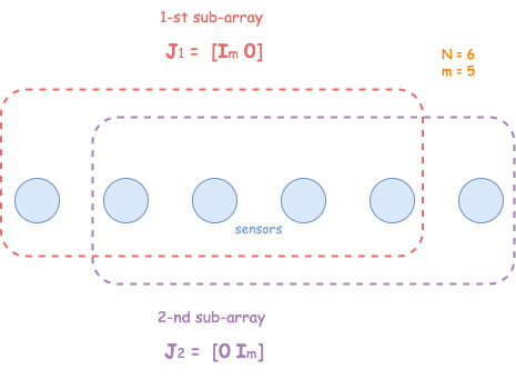
The weight vector \mathbf a(\omega_k) has the property that adjacent entries are related.[\mathbf{a}(\omega_k)]{m+1} = e^{-j\omega_k} [\mathbf{a}(\omega_k)]{m} For the whole vector \mathbf a(\omega_k) , the equation introduces two selection matrices \mathbf{J}1 and \mathbf{J}2 : \mathbf J_1 = [\mathbf I{M-1} \quad \mathbf 0] and \mathbf J_2 = [\mathbf 0 \quad \mathbf I{M-1}]. Here, \mathbf I_{M-1} is an identity matrix of size (M-1) and \mathbf 0 is a vector of M-1 zeros.

The vector \mathbf J_1 \mathbf a(\omega_k) [\mathbf J_2 \mathbf a(\omega_k)] contains all elements of \mathbf a(\omega_k) except the last [first] one. Thus, \mathbf J_2 \mathbf a(\omega_k) = e^{-j\omega_k} \mathbf J_1 \mathbf a(\omega_k) and\mathbf J_2 \mathbf A = \mathbf J_1 \mathbf A \mathbf H ,\quad\text{where}\quad {\mathbf {H}} := \begin{bmatrix} e^{-j\omega_1} & \ & e^{-j\omega_2} \ & & \ddots \ & & & e^{-j\omega_K} \end{bmatrix} .The above relation is the first major observation required for ESPRIT. The second major observation concerns the signal subspace that can be computed from the output signals.

Signal subspace

The singular value decomposition (SVD) of \mathbf Y is given as\mathbf{Y} = \mathbf U \mathbf \Sigma \mathbf V^\dagger where \mathbf U \in\mathbb C^{M\times M} and \mathbf V \in \mathbb C^{T\times T} are unitary matrices and \mathbf \Sigma is a diagonal matrix of size M \times T, that holds the singular values from the largest (top left) in descending order. The operator \dagger denotes the complex-conjugate transpose (Hermitian transpose).

Let us assume that T \geq M. Notice that we have K input signals. If there was no noise, there would only be K non-zero singular values. We assume that the K largest singular values stem from these input signals and other singular values are presumed to stem from noise. The matrices in the SVD of \mathbf Y can be partitioned into submatrices, where some submatrices correspond to the signal subspace and some correspond to the noise subspace. \begin{aligned} \mathbf{U} = \begin{bmatrix} \mathbf{U}\mathrm{S} & \mathbf{U}\mathrm{N} \end{bmatrix}, & & \mathbf{\Sigma} = \begin{bmatrix} \mathbf{\Sigma}\mathrm{S} & \mathbf{0} & \mathbf{0} \ \mathbf{0} & \mathbf{\Sigma}\mathrm{N} & \mathbf{0} \end{bmatrix}, & & \mathbf{V} = \begin{bmatrix} \mathbf{V}\mathrm{S} & \mathbf{V}\mathrm{N} & \mathbf{V}\mathrm{0} \end{bmatrix} \end{aligned}, where \mathbf{U}\mathrm{S} \in \mathbb{C}^{M \times K} and \mathbf{V}\mathrm{S} \in \mathbb{C}^{T \times K} contain the first K columns of \mathbf U and \mathbf V , respectively and \mathbf{\Sigma}\mathrm{S} \in \mathbb{C}^{K \times K} is a diagonal matrix comprising the K largest singular values.

Thus, The SVD can be written as \mathbf{Y} = \mathbf U_\mathrm{S} \mathbf \Sigma_\mathrm{S} \mathbf V_\mathrm{S}^\dagger

• \mathbf U_\mathrm{N} \mathbf \Sigma_\mathrm{N} \mathbf V_\mathrm{N}^\dagger , where \mathbf{U}\mathrm{S} , ⁣\mathbf{V}\mathrm{S} , and \mathbf{\Sigma}\mathrm{S} represent the contribution of the input signal x_k[t] to \mathbf Y . We term \mathbf{U}\mathrm{S} the signal subspace. In contrast, \mathbf{U}\mathrm{N} , \mathbf{V}\mathrm{ N } , and \mathbf{\Sigma}_\mathrm{N} represent the contribution of noise n_m[ t ] to \mathbf Y .

Hence, from the system model, we can write \mathbf{A} \mathbf{X} = \mathbf U_\mathrm{S} \mathbf \Sigma_\mathrm{S} \mathbf V_\mathrm{S}^\dagger and \mathbf{N} = \mathbf U_\mathrm{N} \mathbf\Sigma_\mathrm{N} \mathbf V_\mathrm{N}^\dagger . Also, from the former, we can write \mathbf U_\mathrm{S} = \mathbf{A} \mathbf{F}, where {\mathbf F } = \mathbf{X} \mathbf V_\mathrm{S} \mathbf \Sigma_\mathrm{S}^{-1} . In the sequel, it is only important that there exists such an invertible matrix \mathbf F and its actual content will not be important.

Note: The signal subspace can also be extracted from the spectral decomposition of the auto-correlation matrix of the measurements, which is estimated as\mathbf{R}_\mathrm{YY}

\frac{1}{T} \sum_{t=1}^T \mathbf{y}[t] \mathbf{y}[t] ^\dagger =\frac{1}{T} \mathbf{Y} \mathbf{Y}^\dagger

\frac{1}{T} \mathbf U {\mathbf \Sigma \mathbf \Sigma^\dagger} \mathbf U^\dagger

\frac{1}{T} \mathbf U_\mathrm{S} \mathbf \Sigma_\mathrm{S}^2 \mathbf U_\mathrm{S}^\dagger + \frac{1}{T} \mathbf U_\mathrm{N} \mathbf \Sigma_\mathrm{N}^2 \mathbf U_\mathrm{N}^\dagger.

Estimation of radial frequencies

We have established two expressions so far: \mathbf J_2 \mathbf A = \mathbf J_1 \mathbf A \mathbf H and \mathbf U_\mathrm{S} = \mathbf{A} \mathbf{F} . Now, \begin{aligned} \mathbf J_2 \mathbf A = \mathbf J_1 \mathbf A \mathbf H \implies \mathbf J_2 (\mathbf U_\mathrm{S} \mathbf{F}^{-1}) = \mathbf J_1 (\mathbf U_\mathrm{S} \mathbf{F}^{-1}) \mathbf H \implies \mathbf S_2 = \mathbf S_1 \mathbf{P}, \end{aligned} where \mathbf{S}1 = \mathbf J_1 \mathbf U\mathrm{S} and \mathbf{S}2 = \mathbf J_2 \mathbf U\mathrm{S} denote the truncated signal sub spaces, and \mathbf{P} = \mathbf{F}^{-1} \mathbf H \mathbf{F}.The above equation has the form of an eigenvalue decomposition, and the phases of the eigenvalues in the diagonal matrix \mathbf H are used to estimate the radial frequencies.

Thus, after solving for \mathbf P in the relation \mathbf S_2 = \mathbf S_1 \mathbf{P}, we would find the eigenvalues \lambda_1,\ \lambda_2,\ \ldots,\ \lambda_K of \mathbf P, where \lambda_k = \alpha_k \mathrm{e}^{-j \omega_k}, and the radial frequencies \omega_1,\ \omega_2,\ \ldots,\ \omega_K are estimated as the phases (argument) of the eigenvalues.

Remark: In general, \mathbf S_1 is not invertible. One can use the least squares estimate {\mathbf P} = (\mathbf S_1^\dagger {\mathbf S_1})^{-1} \mathbf S_1^\dagger {\mathbf S_2}. An alternative would be the total least squares estimate.

Algorithm summary

Input: Measurements \mathbf{Y} := [,\mathbf{y}[1] ,\ \mathbf{y}[2] ,\ \dots ,\ \mathbf{y}[ T ],] , the number of input signals K (estimate if not already known).

1. Compute the singular value decomposition (SVD) of \mathbf{Y} = \mathbf U \mathbf \Sigma \mathbf V^\dagger and extract the signal subspace \mathbf{U}_\mathrm{S} \in \mathbb{C}^{M \times K} as the first K columns of \mathbf U .
2. Compute \mathbf{S}1 = \mathbf J_1 \mathbf U\mathrm{S} and \mathbf{S}2 = \mathbf J_2 \mathbf U\mathrm{S} , where \mathbf J_1 = [\mathbf I_{M-1} \quad \mathbf 0] and \mathbf J_2 = [\mathbf 0 \quad \mathbf I_{M-1}] .
3. Solve for \mathbf{P} in \mathbf S_2 = \mathbf S_1 \mathbf{P} (see the remark above).
4. Compute the eigenvalues \lambda_1, \lambda_2, \ldots, \lambda_K of \mathbf{P} .
5. The phases of the eigenvalues \lambda_k = \alpha_k \mathrm{e}^{-j \omega_k} provide the radial frequencies \omega_k , i.e., \omega_k = -\arg \lambda_k .

Notes

Choice of selection matrices

In the derivation above, the selection matrices \mathbf J_1 = [\mathbf I_{M-1} \quad \mathbf 0] and \mathbf J_2 = [\mathbf 0 \quad \mathbf I_{M-1}] were used. However, any appropriate matrices \mathbf J_1 and \mathbf{J}_2 may be used as long as the rotational invariance ( i.e., \mathbf J_2 \mathbf a(\omega_k) = e^{-j\omega_k} \mathbf J_1 \mathbf a(\omega_k) ) , or some generalization of it (see below) holds; accordingly, the matrices \mathbf J_1 \mathbf A and \mathbf J_2 \mathbf A may contain any rows of \mathbf A .

Generalized rotational invariance

The rotational invariance used in the derivation may be generalized. So far, the matrix \mathbf H has been defined to be a diagonal matrix that stores the sought-after complex exponentials on its main diagonal. However, \mathbf H may also exhibit some other structure. For instance, it may be an upper triangular matrix. In this case, \mathbf{P} = \mathbf{F}^{-1} \mathbf H \mathbf{F}constitutes a triangularization of \mathbf P.

References

References

1. (1985). "Nineteenth Asilomar Conference on Circuits, Systems and Computers".
2. Volodymyr Vasylyshyn. The direction of arrival estimation using ESPRIT with sparse arrays.// Proc. 2009 European Radar Conference (EuRAD). – 30 Sept.-2 Oct. 2009. - Pp. 246 - 249. - [https://ieeexplore.ieee.org/abstract/document/5307000]
3. (2014). "An ESPRIT-Based Approach for 2-D Localization of Incoherently Distributed Sources in Massive MIMO Systems". IEEE Journal of Selected Topics in Signal Processing.