Maxwell–Boltzmann distribution

Distribution function

For a system containing a large number of identical non-interacting, non-relativistic classical particles in thermodynamic equilibrium, the fraction of the particles within an infinitesimal element of the three-dimensional velocity space dv, centered on a velocity vector \mathbf{v} of magnitude v, is given by f(\mathbf{v}) ~ d^3\mathbf{v} = \biggl[\frac{m}{2 \pi k_\text{B}T}\biggr]^ , \exp\left(-\frac{mv^2}{2k_\text{B}T}\right) ~ d^3\mathbf{v}, where:

• m is the particle mass;
• kB is the Boltzmann constant;
• T is thermodynamic temperature;
• f(\mathbf{v}) is a probability distribution function, properly normalized so that \int f(\mathbf{v}) , d^3\mathbf{v} over all velocities is unity.

One can write the element of velocity space as d^3\mathbf{v} = dv_x , dv_y , dv_z, for velocities in a standard Cartesian coordinate system, or as d^3\mathbf{v} = v^2 , dv , d\Omega in a standard spherical coordinate system, where d\Omega = \sin{v_\theta} ~ dv_\phi ~ dv_\theta is an element of solid angle and v^2 = |\mathbf{v}|^2 = v_x^2 + v_y^2 + v_z^2.

Alternately, the distribution function can also be written in momentum space asf(\mathbf{p}) , d^3\mathbf{p} = \left[\frac{1}{2\pi m k_\text{B}T}\right]^{3/2} \exp\left(-\frac{p^2}{2 m k_\text{B}T}\right) , d^3\mathbf{p}where \mathbf{p} = m \mathbf{v} is the momentum vector.

The Maxwellian distribution function for particles moving in only one direction, if this direction is x, is a normal distribution with a standard deviation of \sqrt{k_\text{B}T / m}: f(v_x) ~dv_x = \sqrt{\frac{m}{2 \pi k_\text{B}T}} , \exp\left(-\frac{mv_x^2}{2k_\text{B}T}\right) ~ dv_x, which can be obtained by integrating the three-dimensional form given above over v and v.

Recognizing the symmetry of f(v), one can integrate over solid angle and write a probability distribution of speeds as the function

f(v) = \biggl[\frac{m}{2 \pi k_\text{B}T}\biggr]^ , 4\pi v^2 \exp\left(-\frac{mv^2}{2k_\text{B}T}\right).

This probability density function gives the probability, per unit speed, of finding the particle with a speed near v. This equation is simply the Maxwell–Boltzmann distribution (given in the infobox) with distribution parameter a = \sqrt{k_\text{B}T/m},. The Maxwell–Boltzmann distribution is equivalent to the chi distribution with three degrees of freedom and scale parameter a = \sqrt{k_\text{B}T/m},.

The simplest ordinary differential equation satisfied by the distribution is: \begin{align} 0 &= k_\text{B}T v f'(v) + f(v) \left(mv^2 - 2k_\text{B}T\right), \[4pt] f(1) &= \sqrt{\frac{2}{\pi}} , \biggl[\frac{m}{k_\text{B} T}\biggr]^{3/2} \exp\left(-\frac{m}{2k_\text{B}T}\right); \end{align}

or in unitless presentation: \begin{align} 0 &= a^2 x f'(x) + \left(x^2-2 a^2\right) f(x), \[4pt] f(1) &= \frac{1}{a^3} \sqrt{\frac{2}{\pi }} \exp\left(-\frac{1}{2 a^2} \right). \end{align} With the Darwin–Fowler method of mean values, the Maxwell–Boltzmann distribution is obtained as an exact result.

Relaxation to the 2D Maxwell–Boltzmann distribution

For particles confined to move in a plane, the speed distribution is given by

P(s

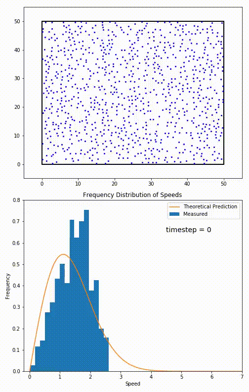
This distribution is used for describing systems in equilibrium. However, most systems do not start out in their equilibrium state. The evolution of a system towards its equilibrium state is governed by the Boltzmann equation. The equation predicts that for short range interactions, the equilibrium velocity distribution will follow a Maxwell–Boltzmann distribution. To the right is a molecular dynamics (MD) simulation in which 900 hard sphere particles are constrained to move in a rectangle. They interact via perfectly elastic collisions. The system is initialized out of equilibrium, but the velocity distribution (in blue) quickly converges to the 2D Maxwell–Boltzmann distribution (in orange).

Typical speeds

The mean speed \langle v \rangle, most probable speed (mode) vp, and root-mean-square speed \sqrt{\langle v^2 \rangle} can be obtained from properties of the Maxwell distribution.

This works well for nearly ideal, monatomic gases like helium, but also for molecular gases like diatomic oxygen. This is because despite the larger heat capacity (larger internal energy at the same temperature) due to their larger number of degrees of freedom, their translational kinetic energy (and thus their speed) is unchanged.

| The most probable speed, vp, is the speed most likely to be possessed by any molecule (of the same mass m) in the system and corresponds to the maximum value or the mode of f(v). To find it, we calculate the derivative set it to zero and solve for v: \frac{df(v)}{dv} = -8\pi \biggl[\frac{m}{2 \pi k_\text{B}T}\biggr]^{3/2} , v , \left[\frac{mv^2}{2k_\text{B}T}-1\right] \exp\left(-\frac{mv^2}{2k_\text{B}T}\right) = 0 with the solution: \frac{mv_\text{p}^2}{2k_\text{B}T} = 1; \quad v_\text{p} = \sqrt{ \frac{2k_\text{B}T}{m} } = \sqrt{ \frac{2RT}{M} } where:

• R is the gas constant;
• M is molar mass of the substance, and thus may be calculated as a product of particle mass, m, and Avogadro constant, NA: M = m N_\mathrm{A}. For diatomic nitrogen (, the primary component of air)The calculation is unaffected by the nitrogen being diatomic. Despite the larger heat capacity (larger internal energy at the same temperature) of diatomic gases relative to monatomic gases, due to their larger number of degrees of freedom, \frac{3RT}{M_\text{m}} is still the mean translational kinetic energy. Nitrogen being diatomic only affects the value of the molar mass . See e.g. K. Prakashan, Engineering Physics (2001), 2.278. at room temperature (), this gives v_\text{p} \approx \sqrt{\frac{2 \cdot 8.31, \mathrm{J {\cdot} {mol}^{-1} K^{-1}} \ 300, \mathrm{K}}{0.028, \mathrm{ {kg} {\cdot} {mol}^{-1} }}} \approx 422, \mathrm{m/s}. | The mean speed is the expected value of the speed distribution, setting b= \frac{1}{2a^2} = \frac{m}{2k_\text{B}T}: \begin{align} \langle v \rangle &= \int_0^{\infty} v , f(v) , dv \[1ex] &= 4\pi \left[ \frac{b}{\pi} \right]^{3/2} \int_0^\infty v^3 e^{-b v^2} dv = 4\pi \left[ \frac{b}{\pi} \right]^{3/2} \frac{1}{2b^2} \[1.4ex] &= \sqrt{\frac{4}{\pi b}} = \sqrt{ \frac{8k_\text{B}T}{\pi m}} = \sqrt{ \frac{8RT}{\pi M}} = \frac{2}{\sqrt{\pi}} v_\text{p} \end{align} | The mean square speed \langle v^2 \rangle is the second-order raw moment of the speed distribution. The "root mean square speed" v_\text{rms} is the square root of the mean square speed, corresponding to the speed of a particle with average kinetic energy, setting b = \frac{1}{2a^2} = \frac{m}{2k_\text{B}T}: \begin{align} v_\text{rms} & = \sqrt{\langle v^2 \rangle} = \left[\int_0^{\infty} v^2 , f(v) , dv \right]^{1/2} \[1ex] & = \left[ 4 \pi \left (\frac{b}{\pi } \right)^{3/2} \int_{0}^{\infty} v^4 e^{-bv^2} dv\right]^{1/2} \[1ex] & = \left[ 4 \pi \left (\frac{b}{\pi}\right )^{3/2} \frac{3}{8} \left(\frac{\pi}{b^5}\right)^{1/2} \right]^{1/2} = \sqrt{ \frac{3}{2b} } \[1ex] &= \sqrt { \frac{3k_\text{B}T}{m}} = \sqrt { \frac{3RT}{M} } = \sqrt{ \frac{3}{2} } v_\text{p} \end{align}

In summary, the typical speeds are related as follows: v_\text{p} \approx 88.6%\ \langle v \rangle

The root mean square speed is directly related to the speed of sound c in the gas, by c = \sqrt{\frac{\gamma}{3}} \ v_\mathrm{rms} = \sqrt{\frac{f+2}{3f}}\ v_\mathrm{rms} = \sqrt{\frac{f+2}{2f}}\ v_\text{p} , where \gamma = 1 + \frac{2}{f} is the adiabatic index, f is the number of degrees of freedom of the individual gas molecule. For the example above, diatomic nitrogen (approximating air) at , f = 5Nitrogen at room temperature is considered a "rigid" diatomic gas, with two rotational degrees of freedom additional to the three translational ones, and the vibrational degree of freedom not accessible. and c = \sqrt{\frac{7}{15}}v_\mathrm{rms} \approx 68%\ v_\mathrm{rms} \approx 84%\ v_\text{p} \approx 353\ \mathrm{m/s}, the true value for air can be approximated by using the average molar weight of air (), yielding at (corrections for variable humidity are of the order of 0.1% to 0.6%).

The average relative velocity \begin{align} v_\text{rel} \equiv \langle |\mathbf{v}_1 - \mathbf{v}_2| \rangle &= \int ! d^3\mathbf{v}_1 , d^3\mathbf{v}_2 \left|\mathbf{v}_1 - \mathbf{v}2\right| f(\mathbf{v}1) f(\mathbf{v}2) \[2pt] &= \frac{4}{\sqrt{\pi}}\sqrt{\frac{k\text{B}T}{m}} = \sqrt{2}\langle v \rangle \end{align} where the three-dimensional velocity distribution is f(\mathbf{v}) \equiv \left[\frac{2\pi k\text{B}T}{m}\right]^{-3/2} \exp\left(-\frac{1}{2}\frac{m\mathbf{v}^2}{k\text{B}T} \right).

The integral can easily be done by changing to coordinates \mathbf{u} = \mathbf{v}_1-\mathbf{v}_2 and \mathbf{U} = \tfrac{1}{2}(\mathbf{v}_1 + \mathbf{v}_2).

Limitations

The Maxwell–Boltzmann distribution assumes that the velocities of individual particles are much less than the speed of light, i.e. that T \ll \frac{m c^2}{k_\text{B}}. For electrons, the temperature of electrons must be T_e \ll 5.93 \times 10^9~\mathrm{K}. For distribution of speeds of relativistic particles, see Maxwell–Jüttner distribution.

Derivation and related distributions

Maxwell–Boltzmann statistics

Main article: Maxwell–Boltzmann statistics#Derivations, Boltzmann distribution

The original derivation in 1860 by James Clerk Maxwell was an argument based on molecular collisions of the Kinetic theory of gases as well as certain symmetries in the speed distribution function; Maxwell also gave an early argument that these molecular collisions entail a tendency towards equilibrium. After Maxwell, Ludwig Boltzmann in 1872 also derived the distribution on mechanical grounds and argued that gases should over time tend toward this distribution, due to collisions (see H-theorem). He later (1877) derived the distribution again under the framework of statistical thermodynamics. The derivations in this section are along the lines of Boltzmann's 1877 derivation, starting with result known as Maxwell–Boltzmann statistics (from statistical thermodynamics). Maxwell–Boltzmann statistics gives the average number of particles found in a given single-particle microstate. Under certain assumptions, the logarithm of the fraction of particles in a given microstate is linear in the ratio of the energy of that state to the temperature of the system: there are constants k and C such that, for all i, -\log \left(\frac{N_i}{N}\right) = \frac{1}{k}\cdot\frac{E_i}{T} + C. The assumptions of this equation are that the particles do not interact, and that they are classical; this means that each particle's state can be considered independently from the other particles' states. Additionally, the particles are assumed to be in thermal equilibrium.

This relation can be written as an equation by introducing a normalizing factor: \frac{N_i} N = \frac{ \exp\left(-\frac{E_i}{k_\text{B}T}\right) }{ \displaystyle \sum_j \exp\left(-\tfrac{E_j}{k_\text{B}T}\right) }|}}

where:

• Ni is the expected number of particles in the single-particle microstate i,
• N is the total number of particles in the system,
• Ei is the energy of microstate i,
• the sum over index j takes into account all microstates,
• T is the equilibrium temperature of the system,
• kB is the Boltzmann constant. The denominator in is a normalizing factor so that the ratios N_i:N add up to unity — in other words it is a kind of partition function (for the single-particle system, not the usual partition function of the entire system).

Because velocity and speed are related to energy, Equation () can be used to derive relationships between temperature and the speeds of gas particles. All that is needed is to discover the density of microstates in energy, which is determined by dividing up momentum space into equal sized regions.

Distribution for the momentum vector

The potential energy is taken to be zero, so that all energy is in the form of kinetic energy. The relationship between kinetic energy and momentum for massive non-relativistic particles is

where p2 is the square of the momentum vector . We may therefore rewrite Equation () as:

\frac{N_i}{N} = \frac{1}{Z} \exp \left(-\frac{p_{i, x}^2 + p_{i, y}^2 + p_{i, z}^2}{2m k_\text{B}T}\right) |}}

where:

• Z is the partition function, corresponding to the denominator in ;
• m is the molecular mass of the gas;
• T is the thermodynamic temperature;
• kB is the Boltzmann constant. This distribution of N : N is proportional to the probability density function fp for finding a molecule with these values of momentum components, so:

f_\mathbf{p} (p_x, p_y, p_z) \propto \exp \left(-\frac{p_x^2 + p_y^2 + p_z^2}{2m k_\text{B}T}\right)|}}

The normalizing constant can be determined by recognizing that the probability of a molecule having some momentum must be 1. Integrating the exponential in over all px, py, and pz yields a factor of \iiint_{-\infty}^{+\infty} \exp\left(-\frac{p_x^2 + p_y^2 + p_z^2}{2m k_\text{B}T}\right) dp_x, dp_y, dp_z = \Bigl[ \sqrt{\pi} \sqrt{2m k_\text{B}T} \Bigr]^3

So that the normalized distribution function is: f_\mathbf{p} (p_x, p_y, p_z) = \left[\frac{1}{2\pi m k_\text{B}T}\right]^{3/2} \exp\left(-\frac{p_x^2 + p_y^2 + p_z^2}{2m k_\text{B}T}\right) |cellpadding |border |border colour = #50C878 |background colour = #ECFCF4|ref=6}}

The distribution is seen to be the product of three independent normally distributed variables p_x, p_y, and p_z, with variance m k_\text{B}T. Additionally, it can be seen that the magnitude of momentum will be distributed as a Maxwell–Boltzmann distribution, with a = \sqrt{m k_\text{B}T}. The Maxwell–Boltzmann distribution for the momentum (or equally for the velocities) can be obtained more fundamentally using the H-theorem at equilibrium within the Kinetic theory of gases framework.

Distribution for the energy

The energy distribution is found imposing where d^3 \mathbf p is the infinitesimal phase-space volume of momenta corresponding to the energy interval dE. Making use of the spherical symmetry of the energy-momentum dispersion relation E = \tfrac{| \mathbf p|^2}{2m}, this can be expressed in terms of dE as Using then () in (), and expressing everything in terms of the energy E, we get \begin{align} f_E(E) , dE &= \left[\frac{1}{2\pi m k_\text{B}T}\right]^{3/2} \exp\left(-\frac{E}{k_\text{B}T}\right) 4 \pi m \sqrt{2mE} \ dE \[1ex] &= 2 \sqrt{\frac{E}{\pi}} , \left[\frac{1}{k_\text{B}T}\right]^{3/2} \exp\left(-\frac{E}{k_\text{B}T}\right) , dE \end{align} and finally

f_E(E) = 2 \sqrt{\frac{E}{\pi}} , \left[\frac{1}{k_\text{B}T}\right]^{3/2} \exp\left(-\frac{E}{k_\text{B}T} \right) |cellpadding |border |border colour = #50C878 |background colour = #ECFCF4|ref=9}}

Since the energy is proportional to the sum of the squares of the three normally distributed momentum components, this energy distribution can be written equivalently as a gamma distribution, using a shape parameter, k_\text{shape} = 3/2 and a scale parameter, \theta_\text{scale} = k_\text{B}T.

Using the equipartition theorem, given that the energy is evenly distributed among all three degrees of freedom in equilibrium, we can also split f_E(E) , dE into a set of chi-squared distributions, where the energy per degree of freedom, ε is distributed as a chi-squared distribution with one degree of freedom, f_\varepsilon(\varepsilon),d\varepsilon = \sqrt{\frac{1}{\pi\varepsilon k_\text{B}T}} ~ \exp\left(-\frac{\varepsilon}{k_\text{B}T}\right),d\varepsilon

At equilibrium, this distribution will hold true for any number of degrees of freedom. For example, if the particles are rigid mass dipoles of fixed dipole moment, they will have three translational degrees of freedom and two additional rotational degrees of freedom. The energy in each degree of freedom will be described according to the above chi-squared distribution with one degree of freedom, and the total energy will be distributed according to a chi-squared distribution with five degrees of freedom. This has implications in the theory of the specific heat of a gas.

Distribution for the velocity vector

Recognizing that the velocity probability density fv is proportional to the momentum probability density function by

f_\mathbf{v} d^3\mathbf{v} = f_\mathbf{p} \left(\frac{dp}{dv}\right)^3 d^3\mathbf{v}

and using we get

f_\mathbf{v} (v_x, v_y, v_z) = \biggl[\frac{m}{2\pi k_\text{B}T} \biggr]^{3/2} \exp\left(-\frac{m\left(v_x^2 + v_y^2 + v_z^2\right)}{2 k_\text{B}T}\right) |cellpadding |border |border colour = #50C878 |background colour = #ECFCF4}}

which is the Maxwell–Boltzmann velocity distribution. The probability of finding a particle with velocity in the infinitesimal element [dvx, dvy, dvz] about velocity is

f_\mathbf{v}{\left(v_x, v_y, v_z\right)}, dv_x, dv_y, dv_z.

Like the momentum, this distribution is seen to be the product of three independent normally distributed variables v_x, v_y, and v_z, but with variance k_\text{B}T / m. It can also be seen that the Maxwell–Boltzmann velocity distribution for the vector velocity [vx, vy, vz] is the product of the distributions for each of the three directions: f_\mathbf{v}{\left(v_x, v_y, v_z\right)} = f_v (v_x)f_v (v_y)f_v (v_z) where the distribution for a single direction is f_v (v_i) = \sqrt{\frac{m}{2 \pi k_\text{B}T}} \exp \left(-\frac{mv_i^2}{2k_\text{B}T}\right).

Each component of the velocity vector has a normal distribution with mean \mu_{v_x} = \mu_{v_y} = \mu_{v_z} = 0 and standard deviation \sigma_{v_x} = \sigma_{v_y} = \sigma_{v_z} = \sqrt{k_\text{B}T / m}, so the vector has a 3-dimensional normal distribution, a particular kind of multivariate normal distribution, with mean \mu_{\mathbf{v}} = \mathbf{0} and covariance \Sigma_{\mathbf{v}} = \left(\frac{k_\text{B}T}{m}\right)I, where I is the 3 × 3 identity matrix.

A notable property of the distribution for the velocity vector is direction-independence, which means that velocity components are normally distributed in any selected direction, not only in three base directions x, y, and z.

Distribution for the speed

The Maxwell–Boltzmann distribution for the speed follows immediately from the distribution of the velocity vector, above. Note that the speed is v = \sqrt{v_x^2 + v_y^2 + v_z^2} and the volume element in spherical coordinates dv_x, dv_y, dv_z = v^2 \sin \theta, dv, d\theta, d\phi = v^2 , dv , d\Omega where \phi and \theta are the spherical coordinate angles of the velocity vector. Integration of the probability density function of the velocity over the solid angles d\Omega yields an additional factor of 4\pi. The speed distribution with substitution of the speed for the sum of the squares of the vector components: f (v) = \sqrt{\frac{2}{\pi}} , \biggl[\frac{m}{k_\text{B}T}\biggr]^{3/2} v^2 \exp\left(-\frac{mv^2}{2k_\text{B}T}\right).

In ''n''-dimensional space

In n-dimensional space, Maxwell–Boltzmann distribution becomes: f(\mathbf{v}) ~ d^n\mathbf{v} = \biggl[\frac{m}{2 \pi k_\text{B}T}\biggr]^{n/2} \exp\left(-\frac{m|\mathbf{v}|^2}{2k_\text{B}T}\right) ~d^n\mathbf{v}

Speed distribution becomes: f(v) ~ dv = A \exp\left(-\frac{mv^2}{2k_\text{B} T}\right) v^{n-1} ~ dv where A is a normalizing constant.

The following integral result is useful: \begin{align} \int_{0}^{\infty} v^a \exp\left(-\frac{mv^2}{2k_\text{B} T}\right) dv &= \left[\frac{2k_\text{B} T}{m}\right]^\frac{a+1}{2} \int_{0}^{\infty} e^{-x}x^{a/2} , dx^{1/2} \[2pt] &= \left[\frac{2k_\text{B} T}{m}\right]^\frac{a+1}{2} \int_{0}^{\infty} e^{-x}x^{a/2}\frac{x^{-1/2}}{2} , dx \[2pt] &= \left[\frac{2k_\text{B} T}{m}\right]^\frac{a+1}{2} \frac{\Gamma{\left(\frac{a+1}{2}\right)}}{2} \end{align} where \Gamma(z) is the Gamma function. This result can be used to calculate the moments of speed distribution function: \langle v \rangle = \frac {\displaystyle \int_{0}^{\infty} v \cdot v^{n-1} \exp\left(-\tfrac{mv^2}{2k_\text{B} T}\right) , dv} {\displaystyle \int_{0}^{\infty} v^{n-1} \exp\left(-\tfrac{mv^2}{2k_\text{B} T}\right) , dv} = \sqrt{\frac{2k_\text{B} T}{m}} ~~ \frac{\Gamma{\left(\frac{n+1}{2}\right)}}{\Gamma{\left(\frac{n}{2}\right)}} which is the mean speed itself v_\mathrm{avg} = \langle v \rangle = \sqrt{\frac{2k_\text{B} T}{m}} \ \frac{\Gamma \left(\frac{n+1}{2}\right)}{\Gamma \left(\frac{n}{2}\right)}.

\begin{align} \langle v^2 \rangle &= \frac {\displaystyle\int_{0}^{\infty} v^2 \cdot v^{n-1} \exp\left(-\tfrac{mv^2}{2k_\text{B} T}\right) , dv} {\displaystyle\int_{0}^{\infty} v^{n-1} \exp\left(-\tfrac{mv^2}{2k_\text{B}T}\right) , dv} \[1ex] &= \left[\frac{2k_\text{B}T}{m}\right] \frac{\Gamma {\left(\frac{n+2}{2}\right)}}{\Gamma {\left(\frac{n}{2}\right)}} \[1.2ex] &= \left[\frac{2k_\text{B}T}{m}\right] \frac{n}{2} = \frac{n k_\text{B}T}{m} \end{align} which gives root-mean-square speed v_\text{rms} = \sqrt{\langle v^2 \rangle} = \sqrt{\frac{n k_\text{B}T}{m}}.

The derivative of speed distribution function: \frac{df(v)}{dv} = A \exp\left(-\frac{mv^2}{2k_\text{B}T}\right) \biggl[-\frac{mv}{k_\text{B}T} v^{n-1}+(n-1)v^{n-2}\biggr] = 0

This yields the most probable speed (mode) v_\text{p} = \sqrt{\left(n-1\right) k_\text{B}T/m}.

Extension to real gases

The derivations show that the validity of the Maxwell–Boltzmann velocity distribution is limited to ideal gases. A generalization of the formula to all gases (ideal and real alike) is known, its derivation starts from the fact that the properties of both ideal and real gases must be independent of the direction. The formula obtained contains pV_\text{m} terms instead of RT, where p is the pressure, V_\text{m} is the molar volume of the gas sample:

f(v) = \biggl[\frac{M}{2 \pi pV_\text{m}}\biggr]^ , 4\pi v^2 \exp\left(-\frac{Mv^2}{2pV_\text{m}}\right).

Notes

References

References

1. Mandl, Franz. (2008). "Statistical Physics". John Wiley & Sons.
2. (2008). "Sears and Zemansky's University Physics: With Modern Physics". Pearson, Addison-Wesley.
3. Encyclopaedia of Physics (2nd Edition), [[Rita G. Lerner. R.G. Lerner]], G.L. Trigg, VHC publishers, 1991, {{isbn. 3-527-26954-1 (Verlagsgesellschaft), {{isbn. 0-89573-752-3 (VHC Inc.)
4. N.A. Krall and A.W. Trivelpiece, Principles of Plasma Physics, San Francisco Press, Inc., 1986, among many other texts on basic plasma physics
5. Maxwell, J.C. (1860 A): ''Illustrations of the dynamical theory of gases. Part I. On the motions and collisions of perfectly elastic spheres. The London, Edinburgh, and Dublin Philosophical Magazine and Journal of Science'', 4th Series, vol.19, pp.19–32. [https://www.biodiversitylibrary.org/item/53795#page/33/mode/1up]
6. Maxwell, J.C. (1860 B): ''Illustrations of the dynamical theory of gases. Part II. On the process of diffusion of two or more kinds of moving particles among one another. The London, Edinburgh, and Dublin Philosophical Magazine and Journal of Science'', 4th Ser., vol.20, pp.21–37. [https://www.biodiversitylibrary.org/item/20012#page/37/mode/1up]
7. Müller-Kirsten, H. J. W.. (2013). "Basics of Statistical Physics". [[World Scientific]].
8. (2011). "College Physics, Volume 1". Cengage Learning.
9. (2017). "Maxwell and the normal distribution: A colored story of probability, independence, and tendency towards equilibrium". Studies in History and Philosophy of Modern Physics.
10. Boltzmann, L., "Weitere studien über das Wärmegleichgewicht unter Gasmolekülen." ''Sitzungsberichte der Kaiserlichen Akademie der Wissenschaften in Wien, mathematisch-naturwissenschaftliche Classe'', '''66''', 1872, pp. 275–370.
11. Boltzmann, L., "Über die Beziehung zwischen dem zweiten Hauptsatz der mechanischen Wärmetheorie und der Wahrscheinlichkeitsrechnung respektive den Sätzen über das Wärmegleichgewicht." ''Sitzungsberichte der Kaiserlichen Akademie der Wissenschaften in Wien, Mathematisch-Naturwissenschaftliche Classe''. Abt. II, '''76''', 1877, pp. 373–435. Reprinted in ''Wissenschaftliche Abhandlungen'', Vol. II, pp. 164–223, Leipzig: Barth, 1909. '''Translation available at''': http://crystal.med.upenn.edu/sharp-lab-pdfs/2015SharpMatschinsky_Boltz1877_Entropy17.pdf {{Webarchive. link. (2021-03-05)
12. Parker, Sybil P.. (1993). "McGraw-Hill Encyclopedia of Physics". McGraw-Hill.
13. (2005). "Statistical Thermodynamics: Fundamentals and Applications". Cambridge University Press.
14. (2025). "The ideal gas law: derivations and intellectual background". ChemTexts.
15. Lente, G.. (2025). "Direction independence as a key property to derive a particle speed distribution in real gases". Journal of Mathematical Chemistry.