From Surf Wiki (app.surf) — the open knowledge base
Falkner–Skan boundary layer
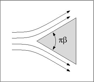
Boundary layer that forms on a wedge
Boundary layer that forms on a wedge
In fluid dynamics, the Falkner–Skan boundary layer (named after Victor Montague Falkner and Sylvia W. Skan) describes the steady two-dimensional laminar boundary layer that forms on a wedge, i.e. flows in which the plate is not parallel to the flow. It is also representative of flow on a flat plate with an imposed pressure gradient along the plate length, a situation often encountered in wind tunnel flow. It is a generalization of the flat plate Blasius boundary layer in which the pressure gradient along the plate is zero.
Prandtl's boundary layer equations
The basis of the Falkner-Skan approach are the Prandtl boundary layer equations. Ludwig Prandtl simplified the equations for fluid flowing along a wall (wedge) by dividing the flow into two areas: one close to the wall dominated by viscosity, and one outside this near-wall boundary layer region where viscosity can be neglected without significant effects on the solution. This means that about half of the terms in the Navier-Stokes equations are negligible in near-wall boundary layer flows (except in a small region near the leading edge of the plate). This reduced set of equations are known as the Prandtl boundary layer equations. For steady incompressible flow with constant viscosity and density, these read:
Mass Continuity: \dfrac{\partial u}{\partial x}+\dfrac{\partial v}{\partial y}=0
x-Momentum: u \dfrac{\partial u}{\partial x} + v \dfrac{\partial u}{\partial y} = - \dfrac{1}{\rho} \dfrac{\partial p}{\partial x} + {\nu} \dfrac{\partial^2 u}{\partial y^2}
y-Momentum: 0 = - \dfrac{\partial p}{\partial y}
Here the coordinate system is chosen with x pointing parallel to the plate in the direction of the flow and the y coordinate pointing towards the free stream, u and v are the x and y velocity components, p is the pressure, \rho is the density and \nu is the kinematic viscosity.
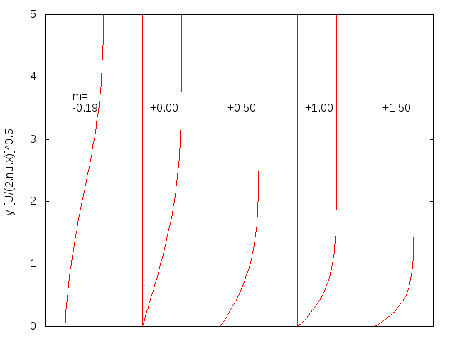
A number of similarity solutions to these equations have been found for various types of flow. Falkner and Skan developed the similarity solution for the case of laminar flow along a wedge in 1930. The term similarity refers to the property that the velocity profiles at different positions in the flow look similar apart from scaling factors in the boundary layer thickness and a characteristic boundary layer velocity. These scaling factors reduce the partial differential equations to a set of relatively easily solved set of ordinary differential equations.
Falkner–Skan equation - First order boundary layer
Source:
Falkner and Skan generalized the Blasius boundary layer by considering a wedge with an angle of \pi \beta / 2 from some uniform velocity field U_0 . Falkner and Skan's first key assumption was that the pressure gradient term in the Prandtl x-momentum equation could be replaced by the differential form of the Bernoulli equation in the high Reynolds number limit. Thus: : -\dfrac{1}{\rho}\dfrac{\partial p}{\partial x} = u_e \dfrac{d u_e}{dx} \quad . Here u_e(x) is the velocity of at the boundary layer edge and is the solution the Euler equations (fluid dynamics) in the outer region.
Having made the Bernoulli equation substitution, Falkner and Skan pointed out that similarity solutions are obtained when the boundary layer thickness and velocity scaling factors are assumed to be simple power functions of x. That is, they assumed the velocity similarity scaling factor is given by:
: u_e(x)= U_0 \left( \frac x L \right)^m \quad ,
where L is the wedge length and m is a dimensionless constant. Falkner and Skan also assumed the boundary layer thickness scaling factor is proportional to:
: \delta (x) ; = ; \sqrt{\frac{2\nu L}{U_0(m+1)}}\left( \frac x L \right)^{(1-m)/2} \quad .
Mass conservation is automatically ensured when the Prandtl momentum boundary layer equations are solved using a stream function approach. The stream function, in terms of the scaling factors, is given by:
: \psi(x,y) ; = ; u_e(x)\delta(x)f(\eta) \quad ,
where \eta = {y}/{\delta (x)} and the velocities are given by:
: u(x,y); = ; \frac,\quad {\rm{and}}\quad v(x,y); = ; - \frac\quad.
This means
:\psi(x,y) ; = ; \sqrt{\frac{2\nu U_0 L}{m+1}}\left( \frac x L \right)^{(m+1)/2} f(\eta) \quad .
The non-dimensionalized Prandtl x-momentum equation using the similarity length and velocity scaling factors together with the stream function based velocities results in an equation known as the Falkner–Skan equation and is given by:
: f'* + f f* + \beta \left[1-(f')^2 \right]=0 \quad ,
where each dash represents differentiation with respect to \eta (Note that another equivalent equation with a different \beta involving an \alpha is sometimes used. This changes f and its derivatives but ultimately results in the same backed-out u(x,y) and v(x,y) solutions). This equation can be solved for certain \beta as an ODE with boundary conditions: :f(0)=f'(0)=0, \quad f'(\infty)=1.
The wedge angle, after some manipulation, is given by:
: \beta = \frac{2m}{m + 1} \quad.
The m = \beta = 0 case corresponds to the Blasius boundary layer solution. When \beta=1, the problem reduces to the Hiemenz flow. Here, m 0 represents a favorable pressure gradient. In 1937 Douglas Hartree showed that physical solutions to the Falkner–Skan equation exist only in the range -0.090429\leq m \leq 2\ (-0.198838\leq\beta\leq 4/3). For more negative values of m, that is, for stronger adverse pressure gradients, all solutions satisfying the boundary conditions at η = 0 have the property that f(η) 1 for a range of values of η. This is physically unacceptable because it implies that the velocity in the boundary layer is greater than in the main flow. Further details may be found in Wilcox (2007).
With the solution for f and its derivatives in hand, the Falkner and Skan velocities become:
: u(x,y) = u_e(x)f' \quad , and : v(x,y) = -\sqrt {\frac {(m+1) \nu U_0 }{2 L} \left( \frac x L \right)^{m-1}} \left(f+\frac{m-1}{m+1}\eta f' \right)\quad .
The Prandtl y-momentum equation can be rearranged to obtain the y-pressure gradient, {\partial p}/{\partial y}, (this is the formula appropriate for the \alpha=1 and \beta=2m/(m+1) case) as : \frac\frac{1}{\rho }\frac; = ; - \frac{1 }(m+1)(3m - 1)f'' + \frac{1 }(m+1)(1 - m)\eta f''' - \frac{1}{4}(m + 1)^2 ff' + \frac{1}{4}(m - 1)^2 \eta f'^2 - \frac{1}{4}(m + 1)(m - 1)\eta ff'' \quad \quad ,
where the displacement thickness, \delta_1, for the Falkner-Skan profile is given by:
:\delta_1 (x)= \left( \frac{2}{m+1}\right)^{1/2} \left( \frac{\nu x}{U}\right)^{1/2} \int_0^\infty (1-f') d\eta
and the shear stress acting at the wedge is given by
:\tau_w (x)= \mu \left( \frac{m+1}{2}\right)^{1/2} \left( \frac{U^3}{\nu x}\right)^{1/2} f''(0)
Compressible Falkner–Skan boundary layer
Source:
Here Falkner–Skan boundary layer with a specified specific enthalpy h at the wall is studied. The density \rho, viscosity \mu and thermal conductivity \kappa are no longer constant here. In the low Mach number approximation, the equation for conservation of mass, momentum and energy become
: \begin{align} \frac{\partial (\rho u)}{\partial x} + \frac{\partial (\rho v)}{\partial y} & = 0,\ \left(u \frac{\partial u}{\partial x} + v \frac{\partial u}{\partial y} \right) & = - \frac{1}{\rho} \frac{dp}{dx} + \frac{1}{\rho}\frac{\partial }{\partial y} \left(\mu\frac{\partial u}{\partial y}\right),\ \rho \left(u \frac{\partial h}{\partial x} + v \frac{\partial h}{\partial y} \right) &= \frac{\partial }{\partial y} \left(\frac{\mu}{Pr} \frac{\partial h}{\partial y} \right) \end{align}
where Pr=c_{p_\infty}\mu_\infty/\kappa_\infty is the Prandtl number with suffix \infty representing properties evaluated at infinity. The boundary conditions become
: u = v = h - h_w(x) = 0 \ \text{for} \ y=0, : u -U = h - h_\infty =0 \ \text{for} \ y=\infty \ \text{or} \ x=0.
Unlike the incompressible boundary layer, similarity solution can exists for only if the transformation
:x\rightarrow c^2 x, \quad y\rightarrow cy, \quad u\rightarrow u, \quad v\rightarrow \frac{v}{c}, \quad h\rightarrow h, \quad \rho\rightarrow \rho, \quad \mu\rightarrow \mu
holds and this is possible only if h_w=\text{constant}.
Howarth transformation
Introducing the self-similar variables using Howarth–Dorodnitsyn transformation
:\eta = \sqrt{\frac{U_o(m+1)}{2\nu_\infty L^m}} x^{\frac{m-1}{2}}\int_0^y \frac{\rho}{\rho_\infty} dy, \quad \psi = \sqrt{\frac{2 U_o \nu_\infty}{(m+1) L^m}} x^{\frac{m+1}{2}} f(\eta), \quad \tilde h(\eta) = \frac{h}{h_\infty}, \quad \tilde h_w = \frac{h_w}{h_\infty}, \quad \tilde \rho = \frac{\rho}{\rho_\infty}, \quad \tilde \mu = \frac{\mu}{\mu_\infty}
the equations reduce to
: \begin{align} (\tilde\rho\tilde \mu f*)' + ff* + \beta [\tilde h - (f')^2] =0, \ (\tilde\rho\tilde\mu \tilde h')' + Prf\tilde h' =0 \end{align}
The equation can be solved once \tilde \rho = \tilde \rho(\tilde h),\ \tilde \mu = \tilde \mu(\tilde h) are specified. The boundary conditions are
:f(0)=f'(0)=\theta(0)-\tilde h_w=f'(\infty)-1=\tilde h(\infty)-1=0.
The commonly used expressions for air are \gamma = 1.4, \ Pr = 0.7, \ \tilde\rho = \tilde h^{-1}, \ \tilde\mu = \tilde h^{2/3}. If c_p is constant, then \tilde h=\tilde \theta = T/T_\infty.
References
References
- Falkner, V. M. and Skan, S. W., (1930). ''[[Aeronautical Research Council Reports and Memoranda. Aero. Res. Coun. Rep. and Mem.]]'' no 1314.
- (1904). "Über Flüssigkeitsbewegung bei sehr kleiner Reibung". Verhandlinger 3. Int. Math. Kongr. Heidelberg.
- Rosenhead, Louis, ed. Laminar boundary layers. Clarendon Press, 1963.
- Falkner, V. M. and Skan, S. W., (1930).
- Falkner, V. M. and Skan, S. W., (1930).
- Schlichting, H., (1979). ''Boundary-Layer Theory'', 7th ed., McGraw-Hill, New York.
- Panton, R., (2013). ''Incompressible Flow'', 4th ed., John Wiley, New Jersey.
- (3 December 1953). "Further Solutions of the Falkner-Skan Equation". Mathematical Transactions of the Cambridge Philosophical Society.
- Schlichting, H., (1979). ''Boundary-Layer Theory'', 7th ed., McGraw-Hill, New York.
- Weyburne, D.. (February 2022). "Aspects of Boundary Layer Theory".
- Lagerstrom, Paco Axel. Laminar flow theory. Princeton University Press, 1996.
This article was imported from Wikipedia and is available under the Creative Commons Attribution-ShareAlike 4.0 License. Content has been adapted to SurfDoc format. Original contributors can be found on the article history page.
Ask Mako anything about Falkner–Skan boundary layer — get instant answers, deeper analysis, and related topics.
Research with MakoFree with your Surf account
Create a free account to save articles, ask Mako questions, and organize your research.
Sign up freeThis content may have been generated or modified by AI. CloudSurf Software LLC is not responsible for the accuracy, completeness, or reliability of AI-generated content. Always verify important information from primary sources.
Report